IV. NEOWISE Data Processing

IV.2. Scan/Frame Pipeline Updates

IV.2.a. Instrumental Calibration

Contents

IV.2.a.i. Overview

The instrumental calibration (ICal) of single-exposure frames from the 4-band (All-Sky) cryogenic phase of the mission was described in detail in section IV.4.a. of the All-Sky Explanatory Supplement. Incremental updates were then made to support the 3-band Cryo (VII.3.b.) and 2-band Post-Cryo (VIII.3.b.) Data Releases. Here we describe updates made to the pixel calibrations and the methods used to remove instrumental signatures from the raw W1,W2 band single-exposure images acquired by the reactivated NEOWISE mission (Dec. 13, 2013 to July 31, 2024). The ICal processing flow is the same as that shown for W1,W2 in Figure 1 of section IV.4.a. in the All-Sky Explanatory Supplement. Cautionary notes for the NEOWISE single-exposure images are outlined in section III.2.

IV.2.a.i.1. Detector (Level-0 Single-Exposure) Trending

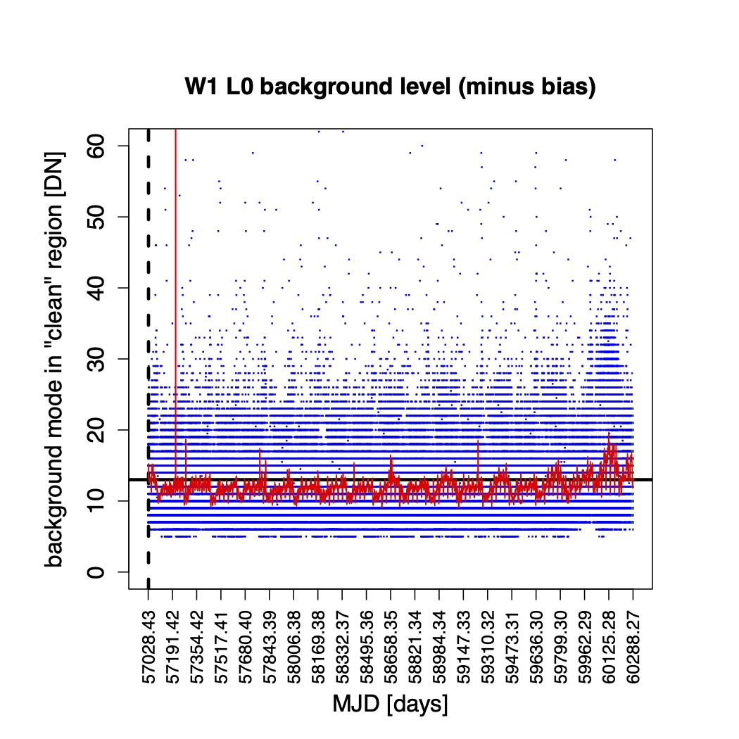
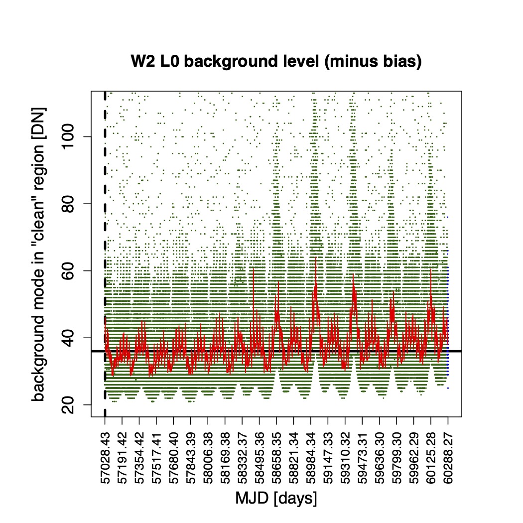
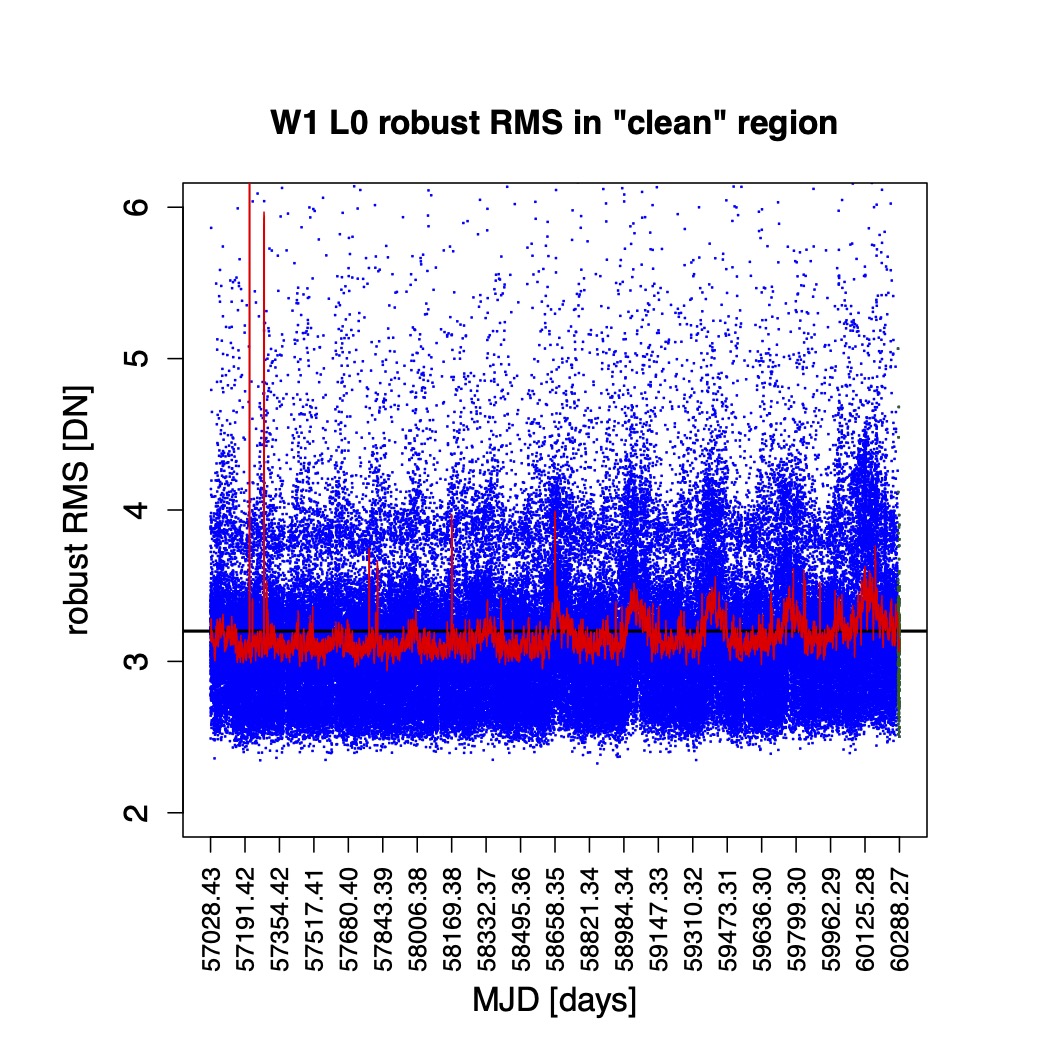
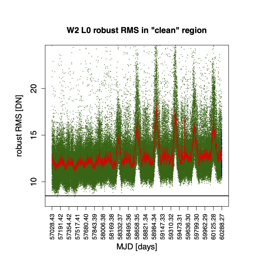
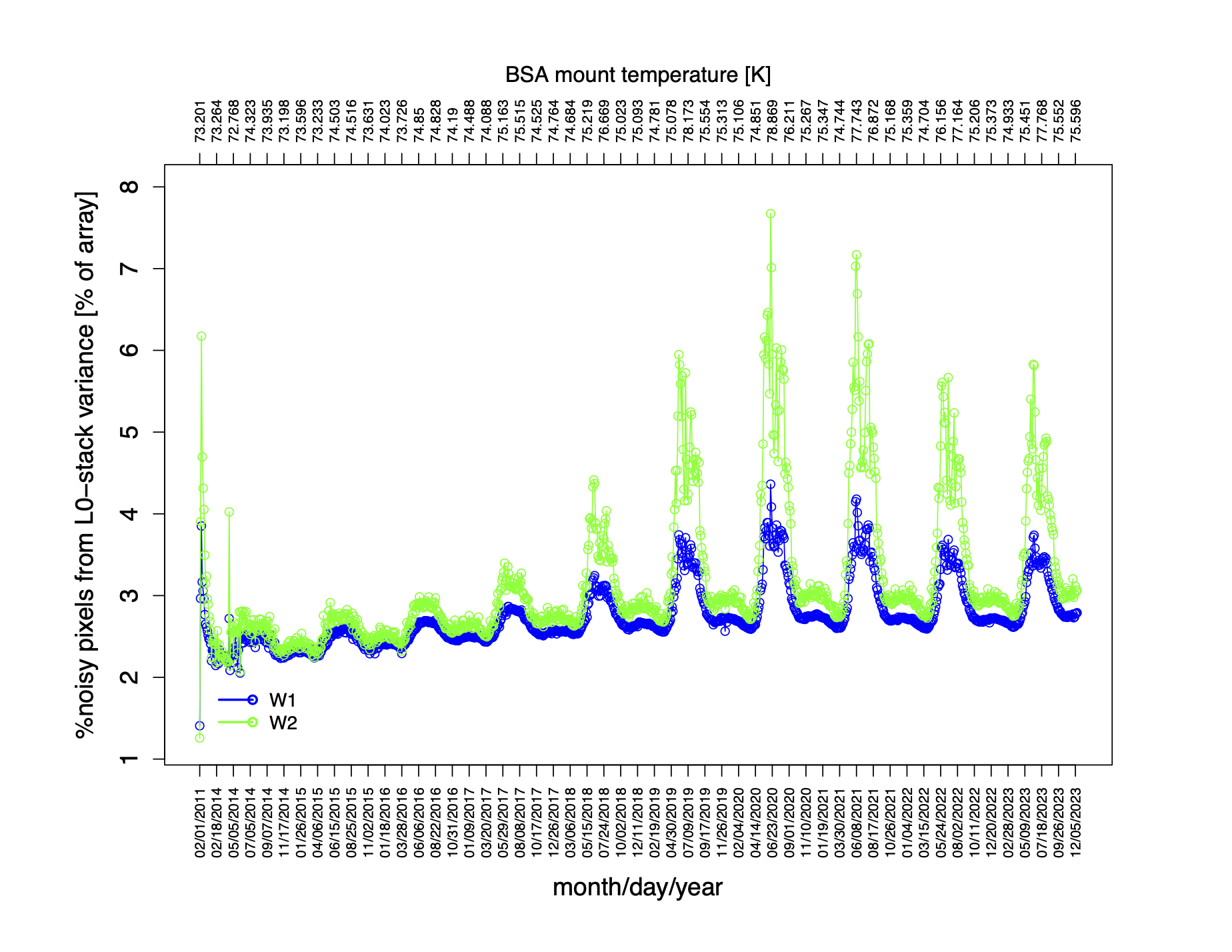
Before outlining our calibration procedures, we summarize some trending metrics that attempt to track general detector performance over the course of the reactivated NEOWISE mission, with comparisons to the original post-cryo phase (Sept. 29, 2010–Feb. 1, 2011). These metrics were derived directly from the raw (Level-0) data with no instrumental calibrations and no pre-processing applied. They are shown as a function of MJD (or date) and beam-splitter assembly (BSA) mount temperature in Figures 1 to 4. The scattering of values at high levels in the background and pixel-RMS levels in Figures 1 and 2 are due to moon-light contamination. The periodic increases in the W1 and W2 backgrounds and pixel-RMS levels are highly correlated with the BSA mount temperatures increases, as shown in the plot of BSA mount temperature in those figures. Figures 1c and 2c more clearly show the impact of temperature on the Level-0 backgrounds and pixel-RMS values.

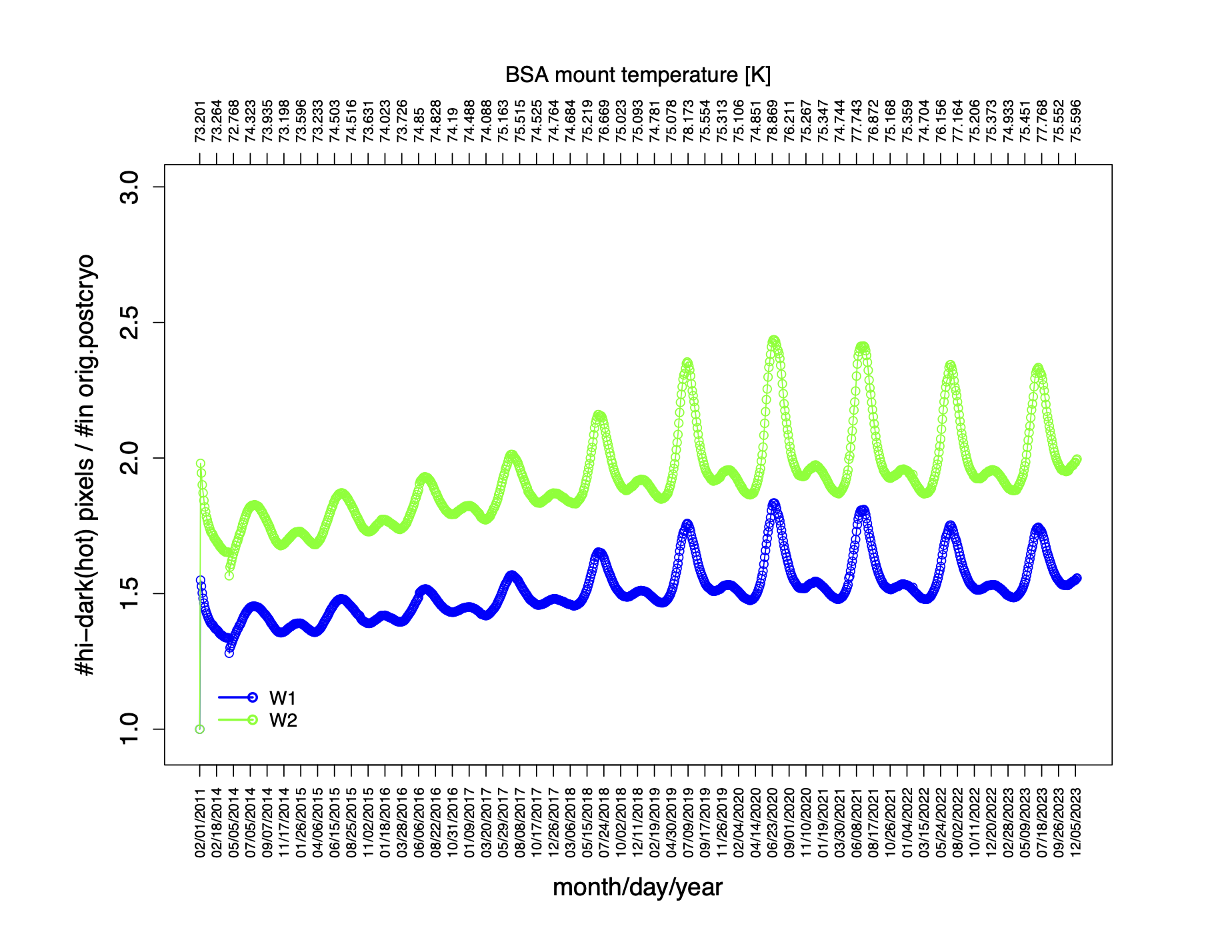
The "hot" pixel fraction trends (Figures 3a, 3b) were made using the dark (relative-bias) calibration products (section IV.2.a.v.) by counting the number of pixels therein that exceeded a fixed threshold of 20 DN. This threshold was determined from examining the high-tails of the dark-pixel histograms. The noisy-pixel fractions (Figures 4a, 4b) were determined from thresholding stacked standard-deviation maps made from Level-0 frames (section IV.2.a.ii.). A fixed threshold of 30 DN was used on these stack-noise maps as inferred from histograms. Note that these thresholds are not those used to create the image-masks for production (i.e., that flag unusable pixels; see below). A large fraction of the hot (high-dark) pixels was found to subtract-out nicely using both the static dark-bias maps (section IV.2.a.v.) and the dynamic sky-offset calibrations (section IV.2.a.ix.). The noisy pixel fractions are closer to what one would mask and declare unusable. The hot pixel trends (Figures 3a, 3b) were normalized to the number of hot pixels at the end of the original post-cryo phase (Feb. 1, 2011). For reference, these numbers (using the same methodology and thresholds) are 132,930 for W1 and 174,976 for W2.

Overall, both the W1 and W2 band detectors performed just as well in terms of sensitivity as in the original post-cryo phase when all calibrations were applied (see below). The notable exceptions were that more bad pixels were accumulated following reactivation of the payload from its warm state at the end of 2013, as well as during the final warm-up starting in April 2024. The largest discrepancies were seen with W2 where the number of hot and noisy pixels (Figures 3a, 4a) increased by a factor of ~ 1.8 on average, compared to ~1.4 for W1. Again, the final 2024 warm-up exceeded these levels in both bands. This increase in the number of bad (primarily hot) pixels affected the overall Level-0 pixel RMS, particularly in W2 (Figure 2), but not necessarily our ability to remove them using the dynamic calibrations (section IV.2.a.ix.). The seasonal variations in the number of hot pixels was closely correlated with the changes in the BSA mount temperature (Figures 3a, 3b). The number of noisy pixels was also correlated with temperature, but it also appears to have been affected by moon avoidance spacecraft maneuvers, the impact of which cause extraordinary excursions in noisy pixel counts, especially and more intensely as the BSA mount temperature rose (Figures 4a and 4b).

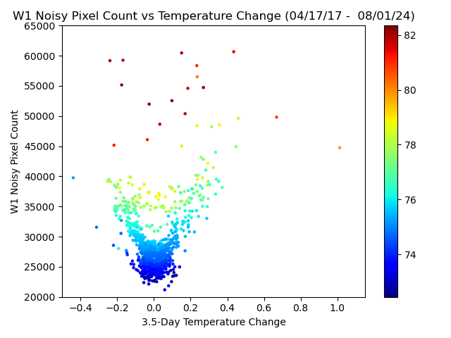
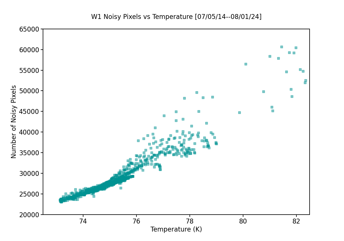
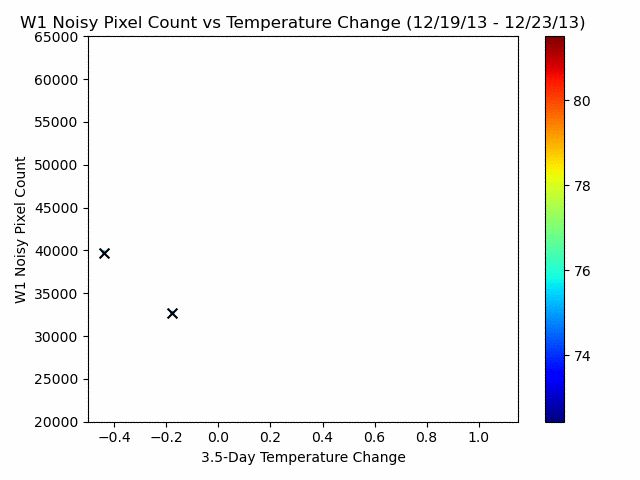
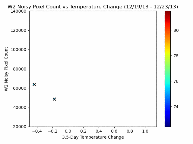
For completeness we also show in Figures 4c and 4d the number of noisy pixels in W1 and W2 as a function of change in the BSA mount temperature, sampled in 3.5-day (half-week) intervals, as well as the noisy pixel count as a function of BSA mount temperature in W1 and W2, in Figures 4e and 4f.

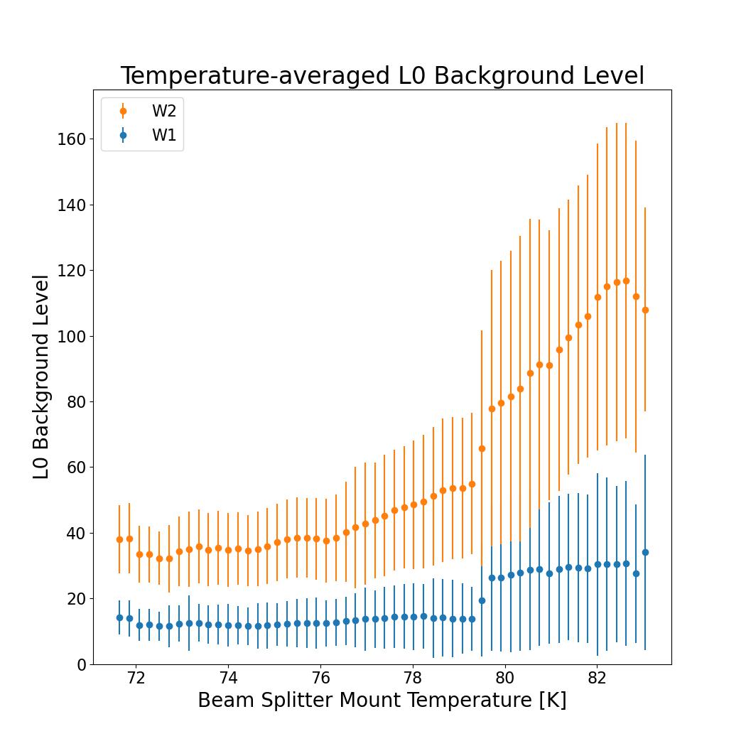Figure 1a - W1 background level in Level-0 single-exposure frames as a function of MJD (Dec. 2014 - July 2024). Backgrounds are pixel mode estimates in a relatively clean region on each array, i.e., with low numbers of bad pixels. The dark blue line is a 7-day running average and the horizontal black line is the median estimate from the last week of original post-cryo (Jan. 25–Feb. 1, 2011). The green line is the temperature of the beam splitter assembly mount. Click to enlarge.	Figure 1b - W2 background level in Level-0 single-exposure frames as a function of MJD (Dec. 2014 - July 2024). Backgrounds are pixel mode estimates in a relatively clean region on each array, i.e., with low numbers of bad pixels. The blue line is a 7-day running average and the horizontal black line are median estimate from the last week of original post-cryo (Jan. 25–Feb. 1, 2011). The green line is the temperature of the beam splitter assembly mount. Click to enlarge.	Figure 1c - The average W1 (blue points) and W2 (red points) background levels in Level-0 single-exposure frames as a function of the beam splitter assembly mount temperature. Click to enlarge. The W1 and W2 data behind this figure can be found in Table 1 (.tbl file, 23 kB) and Table 2 (.tbl file, 23 kB), respectively.

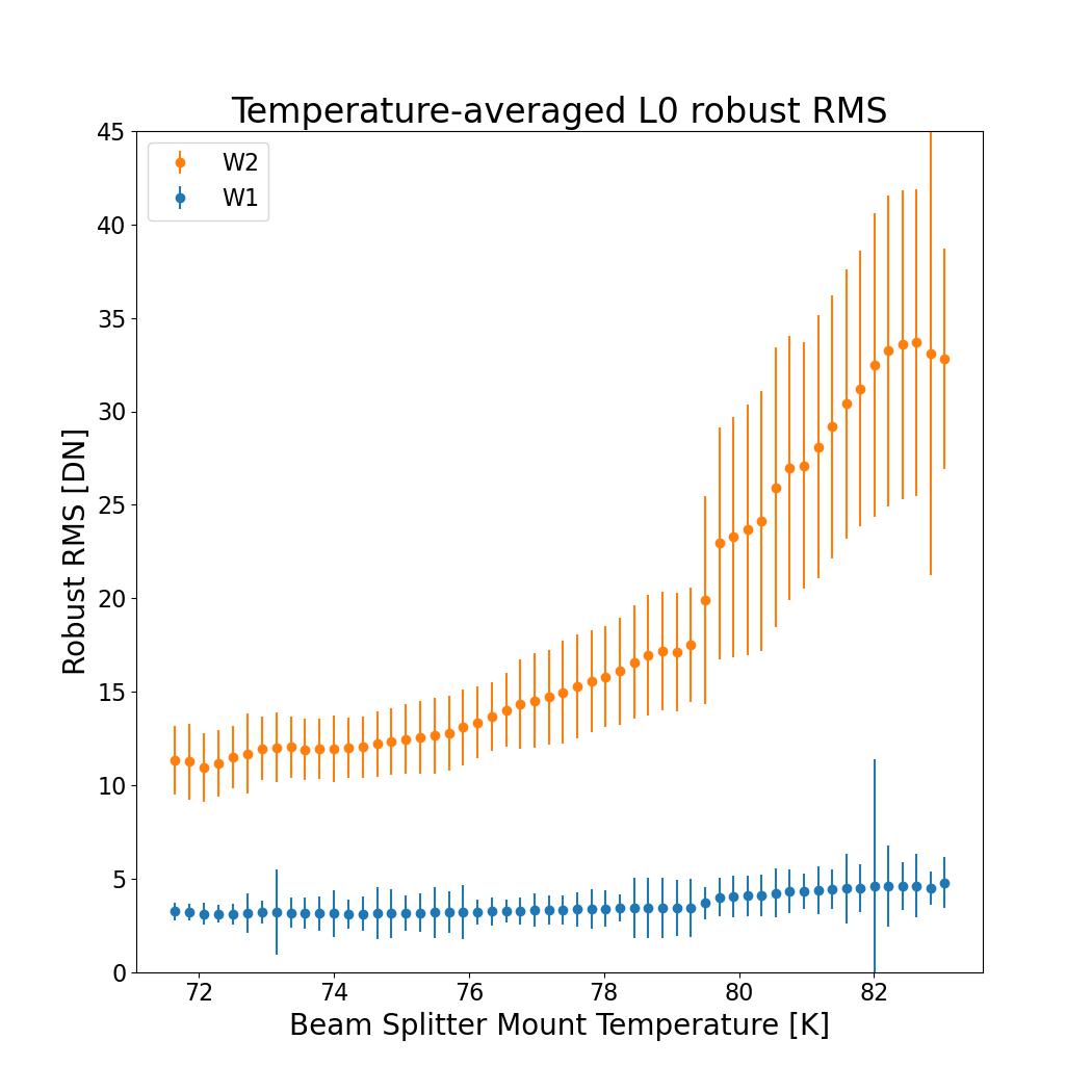Figure 2a - W1 pixel RMS values in Level-0 single-exposure frames as a function of MJD (Dec. 2014 - July 2024). RMS values are robust estimates based on percentiles in a relatively clean region on each array, i.e., with low numbers of bad pixels. The dark blue line is a 7-day running average and horizontal black line is the median estimate from the last week of original post-cryo (Jan. 25 - Feb. 1, 2011). The green line is the temperature of the beam splitter assembly mount. Click to enlarge.	Figure 2b - W2 pixel RMS values in Level-0 single-exposure frames as a function of MJD (Dec. 2014 - July 2024). RMS values are robust estimates based on percentiles in a relatively clean region on each array, i.e., with low numbers of bad pixels. The blue line is a 7-day running average and horizontal black line is the median estimate from the last week of original post-cryo (Jan. 25 - Feb. 1, 2011). The green line is the temperature of the beam splitter assembly mount. Click to enlarge.	Figure 2c - The average W1 (blue points) and W2 (red points) pixel RM values in Level-0 single-exposure frames as a function of the beam splitter assembly mount temperature. Click to enlarge. The W1 and W2 data behind this figure can be found in Table 1 (.tbl file, 23 kB) and Table 2 (.tbl file, 23 kB), respectively.

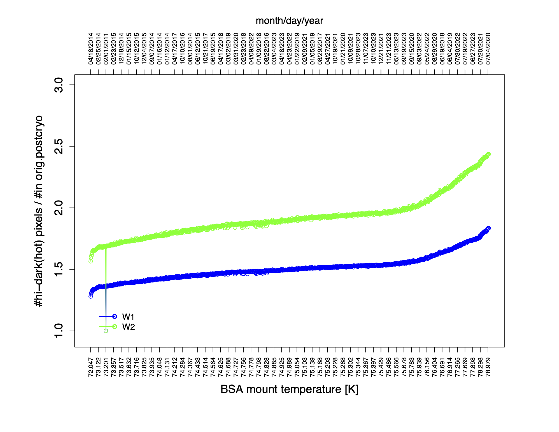Figure 3a - Number of hot (or "high dark") pixels relative to those at the end of the original post-cryo (Feb. 1, 2011) as a function of date where points are separated by time windows spanning 3 to 4 days. The top axis shows the corresponding average BSA mount temperature for each time window. See text for details. Click to enlarge.	Figure 3b - Same as Figure 3a but as a function of BSA mount temperature on the abscissa. The top axis shows the corresponding date for the middle of each time window. See text for details. Click to enlarge.
The data behind this figure can be found in Table 3 (.tbl file, 59 kB).

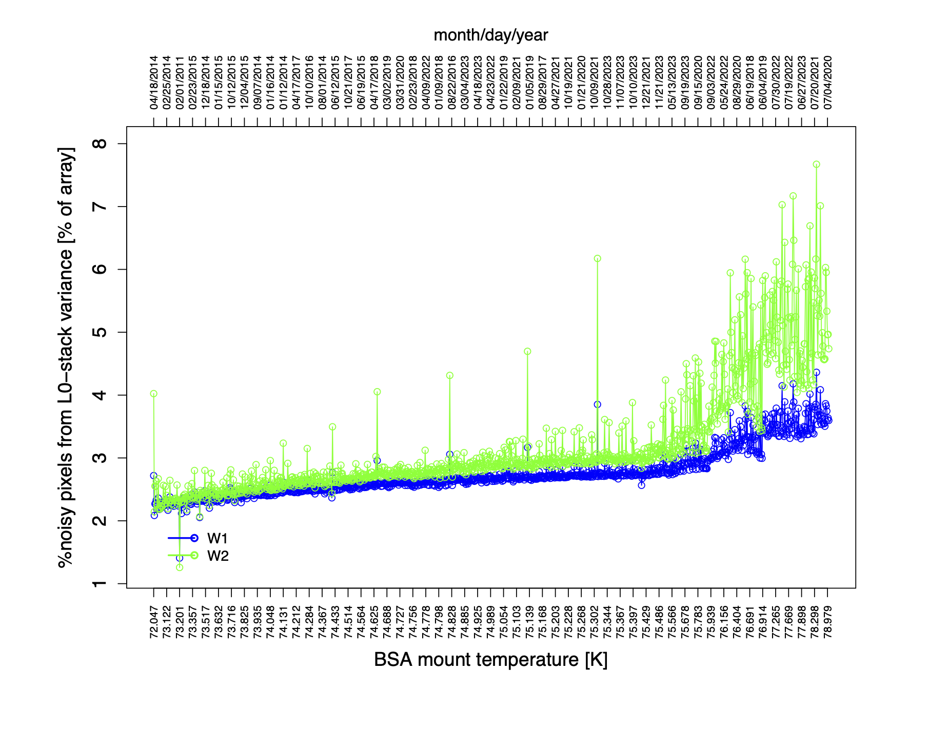Figure 4a - Percentage of noisy pixels over each array as a function of date where points are separated by time windows spanning 3 to 4 days. The first time-point corresponds to the end of original post-cryo (Feb. 1, 2011). The top axis shows the corresponding average BSA mount temperature for each time window. See text for details. Click to enlarge.	Figure 4b - Same as Figure 4a but as a function of BSA mount temperature on the abscissa. The top axis shows the corresponding date for the middle of each time window. See text for details. Click to enlarge.
The data behind this figure can be found in Table 3 (.tbl file, 59 kB).

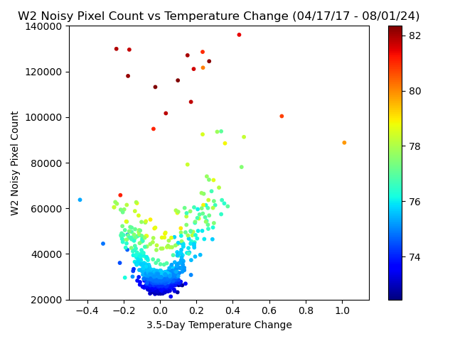Figure 4c - Number of noisy pixels in W1 as a function of temperature change, where points are separated by time windows spanning 3.5 days (half-week). The first time-points correspond to April 17, 2017, up until the end of the mission. The colorbar along the right side shows the corresponding average BSA mount temperature, which is reflected in the colors of the time-points. See text for details. Click to enlarge.	Figure 4d - Same as Figure 4c but in W2. See text for details. Click to enlarge.
A movie of both of these figures is available for W1 as an animated and a MPG file; and same for W2, animated and MPG file.
The data behind this figure can be found in Table 3 (.tbl file, 59 kB).

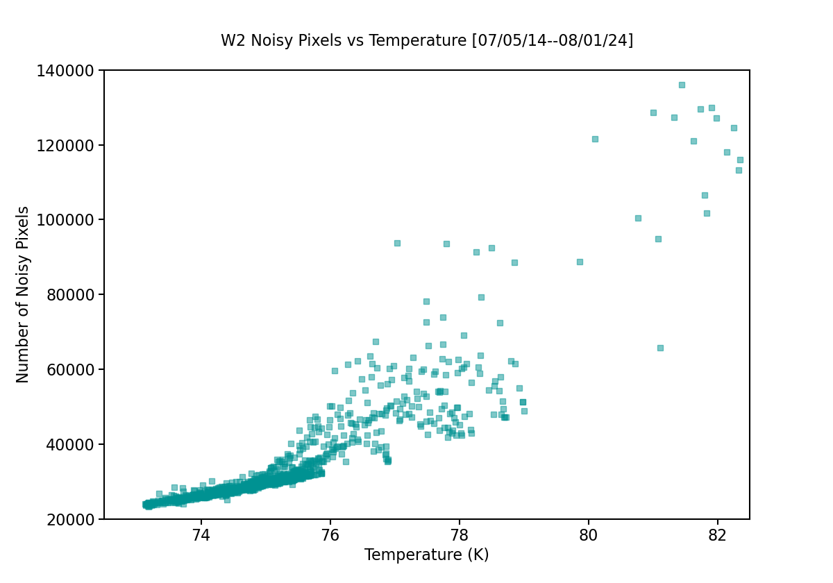Figure 4e - Number of hot (or "high dark") pixels in W1 as a function of BSA mount temperature, in the date range Jul. 5, 2014 through Aug. 1, 2024. The points were sampled in time windows spanning 3.5 days (half-week). See text for details. Click to enlarge.	Figure 4f - Same as Figure 4e but in W2. See text for details. Click to enlarge.
The data behind this figure can be found in Table 3 (.tbl file, 59 kB).

IV.2.a.i.2. Calibration Summary and Intervals

The detector (pixel) calibrations and parameters used in processing the NEOWISE image data are summarized in Table 4. All W1 and W2 calibrations (except for the non-linearity correction) were derived and tuned using the NEOWISE survey data. Also shown in Table 4 is whether the calibration is a static product (derived once and applied throughout the survey with no updates), period-dependent (i.e., progressively updated in response to changes in detector behavior), or dynamic (derived/applied during pipeline processing on a per-frame or per-scan basis).

Table 5 summarizes the calibration period intervals where a fixed set of calibrations were applied. This includes the specific products that were updated in each period since not all products were re-derived. Other relevant tables that track calibration updates and/or detector performance, in general, are Table 6 (bad pixel history) and Table 8 (detector electronic gains and read-noise). There are more calibration intervals early in the NEOWISE survey (18 intervals prior to Feb. 7, 2014) due to the warmer thermal environment and gradual cool-down of the detectors following reactivation.

IV.2.a.i.3. Calibration Procedure, Tracking and Tuning

The detector (pixel) calibrations were periodically updated in response to temperature variations throughout the NEOWISE survey, both during the initial cool-down period following reactivation and then due to subsequent "seasonal" variations. For the latter, systematic trends were observed in the numbers of bad pixels (with lo/hi response, dark signal, and/or with a noisy output in general; see Figures 3 - 4). The decision on whether to update calibrations for a specific period was based on monitoring and analyzing the following four diagnostics:

1. A significant number of residual hot and noisy pixels started to appear in the single-exposure intensity images that were not corrected/masked using static calibrations from the existing/previous interval as well as the ongoing dynamically derived calibrations.
2. Significant residuals started to develop in the relative residual low-spatial frequency relative responsivity maps as determined from spatially-binned differences in source photometry between NEOWISE and the earlier AllWISE Release Catalog.
3. Related to (i): the pixel RMS in single-exposure products (medianed over all exposures per scan) started to deviate significantly.
4. Robust estimates of the ratio of "image-derived pixel RMS" to "noise-model-derived pixel uncertainty" started to deviate significantly from unity. This indicated that the electronic gain and/or read-noise calibrations needed updating (section IV.2.a.iv).

Our (re)calibration procedure is as follows. Further details are given in the sections below.

1. Generate high-spatial frequency (pixel-to-pixel) relative responsivity maps (flat-fields) using raw Level-0 exposures via the "background-gradient" method (section IV.2.a.viii). These maps are then regularized by resetting abnormally low/high pixel values < 0.1 / > 1.8 to unity and tagging them in the frame masks with bit #3 or #4 (section IV.2.a.iii).
2. Generate dark (offset) relative bias-structure maps also using the raw Level-0 exposures (section IV.2.a.viii). These are then regularized by resetting high pixel values > 32,000 DN to the static bias value of 128 DN and tagging them in the frame masks with bit #4 (section IV.2.a.iii).
3. Generate RMS-stack maps from the temporal pixel-dispersion in stacked raw Level-0 exposures (section IV.2.a.iv). These are produced in tandem with the dark/bias calibrations in step 2. Several RMS-stack maps across several consecutive calibration intervals are then combined to produce a single effective RMS-stack map by retaining the maximum RMS value per pixel from all intervals. This gives a "conservative" RMS-stack map that stores information on the noisiest pixels over time, including those that may have been noisy (unstable) for at least one calibration interval in the past. These effective stack-RMS maps are used to generate or update two other calibration products: (i) static calibration masks for tagging noisy pixels (with pixel stack-RMS > 25 DN and bit #1; see section IV.2.a.iii) and (ii) the read-noise sigma maps (step 6 below).
4. Generate the "static" calibration image masks (for the calibration interval of interest) by combining all "bad" pixels from thresholding the products generated in steps 1, 2, and 3.
5. If warranted, compute and validate new electronic gains and read-noise sigmas using pre-processed single-exposure intensity products (see section IV.2.a.iv). The read-noise sigmas are used in step 6.
6. Generate the "static" read-noise maps (for the calibration interval of interest) using the outputs from steps 3 and 5 (see section IV.2.a.iv).
7. Using all new calibrations, process of order 20 recent scans (~ 5000 frames) through the scan-frame pipeline. This includes dynamic calibration. This test provides a first check of the calibration performance. In particular, we collapse all test scans to create residual low-spatial frequency relative responsivity maps determined from spatially-binned differences in source photometry between NEOWISE and the AllWISE Release Catalog. These maps are examined for excess (spatially extended) residuals.
8. If significant residuals are found in the residual low-spatial frequency relative responsivity maps from step 7, we augment the high-spatial frequency responsivity maps from step 1 by multiplying them with the low-frequency responsivity maps and renormalizing to create new flat-field calibrations. The goal here is to remove (or minimize) any low-spatial frequency residual patterns seen in the spatially binned photometric differences.
9. Reprocess the test scans from step 7 and regenerate the residual low-spatial frequency relative responsivity maps to validate the flat-fielding performance. If all is sufficiently flat (to 1% or better), we proceed to step 10, otherwise, we iterate steps 8 and 9 until any significant systematic residuals disappear. Note: this augmentation of the high-frequency responsivity maps using photometrically derived responsivity maps was performed towards the end of year 1 of NEOWISE and continued throughout year 2. For most of year 1, any low-frequency responsivity residuals (typically of order 3 to 5%) were not corrected. See section IV.2.a.viii.1 for details.
10. Compute and update the pixel-uncertainty scaling factors (section IV.2.a.iv) from analyzing the pixel-RMSs and noise-model uncertainty estimates in the single-exposure products. If the gain and read-noise values were estimated correctly, these scaling factors should be close to unity for the calibration interval of interest. At times, however, these values drifted, and instead of re-deriving the electronic gain and read-noise (which are computationally expensive), we updated the pixel-uncertainty scaling factors instead.

IV.2.a.ii. Bad-pixel Masking and Saturation Tagging

Similar to other (NEO)WISE processing phases, the frame masks are initialized in the ICal pipeline by first copying all information from the "static" calibration mask for the specific band (procedure in section IV.2.a.i.3) into the first 8 bits of a 32-bit buffer (see Table 7). The dynamic bits are then assigned on a per-frame basis according to various conditions encountered as each processing step was applied, e.g., saturated and broken pixels, bad/unreliable linearity corrections, temporally transient bad pixels, and spatial pixel-outlier spikes.

The number and percentages of bad (fatal) pixels tagged in the frame masks are summarized in Table 6. These pixels (along with the dynamically set saturated pixels) are set to NaN in the single-exposure intensity and uncertainty frames during processing (see section IV.2.a.iii). These NaN'd pixels are recognized and omitted from the single-exposure photometric measurements downstream. These fatal pixels are predominately those tagged as generally "noisy" (or unstable) for the specific calibration interval (Figure 4 and section IV.2.a.i.3), but they also include permanently bad pixels tagged with a very low or high responsivity, dark current, or an abnormal non-linear response. For comparison, the number of bad (fatal) pixels towards the end of the original post-cryo phase (Jan. 25–Feb. 1, 2011), assuming the same thresholds, was a factor of ~1.8 lower for both bands than reported in Table 6.

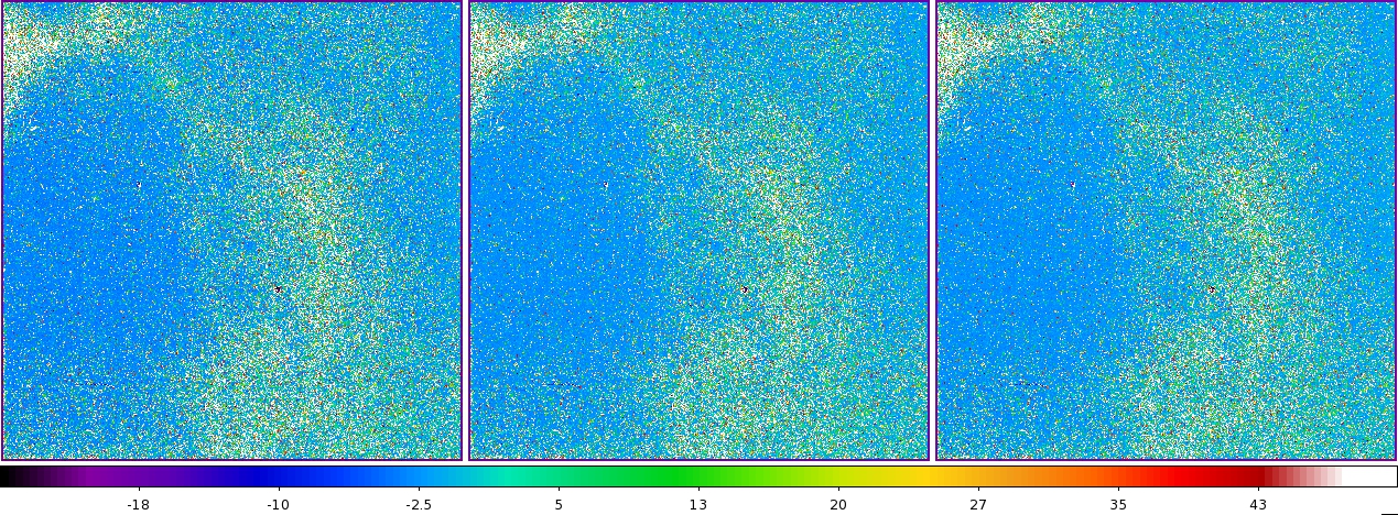
Figures 5a and 5b show the static calibration image masks for W1 and W2 respectively, for three intervals during year 1 of NEOWISE. The largest temporal changes were for W2, owing to its greater sensitivity to the ambient thermal (dark) background. This background was highest soon after the reactivation of the spacecraft in December 2013.

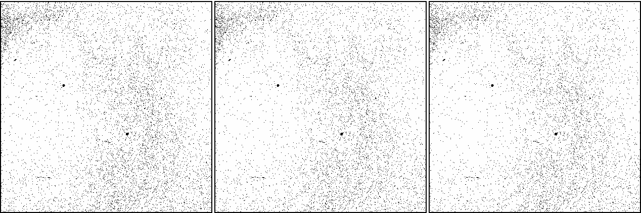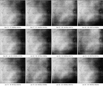
Figure 5a - W1 masks showing bad pixel locations that are set to NaN in instrumentally-calibrated single-exposure products for three different periods during NEOWISE: Dec. 13, 2013 (left); June 4, 2014 (middle); Dec. 9, 2014 (right). Click to enlarge.

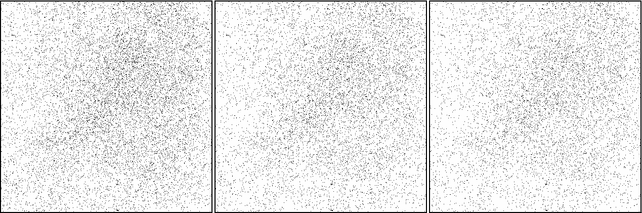Figure 5b - W2 masks showing bad pixel locations that are set to NaN in instrumentally-calibrated single-exposure products for three different periods during NEOWISE: Dec. 13, 2013 (left); June 4, 2014 (middle); Dec. 9, 2014 (right). Click to enlarge.

Bits 9 to 19 in Table 7 refer to the dynamically tagged saturation bits according to values encoded in the raw Level-0 frames set on board the payload (the DEB processing unit). This range reflects the readout sample number in the ramp where the signal first saturates, i.e., hits the maximum of 16,383 DN after A/D conversion in the FEB processing unit. The lowest bits, therefore, refer to more severe cases of saturation, as induced by brighter sources. Bits 9 to 18 refer to "soft" saturation while bit 19 refers to "hard" saturation, i.e., the source was so bright that all reads were saturated. Here, the Level-0 pixel values are fixed at the 128 DN bias level.

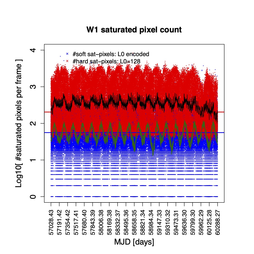
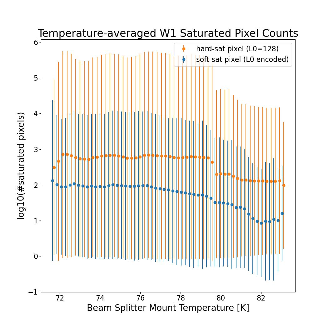
Figure 6 shows the number of soft and hard saturated pixels during the course of the NEOWISE Reactivation survey. The gaps in these plots are due to various spacecraft events that resulted in the loss of survey data (see section I.2.c). The horizontal lines show the corresponding median levels from the end of the original post-cryo (Jan. 25–Feb.1, 2011). With the exception of the number of hard saturated pixel counts in W2, the post-cryo levels are lower than the NEOWISE 7-day running averages. In general, the cyclic pattern seen in the 7-day running averages of the soft saturated counts (dark blue lines) corresponds well with the inverse of the seasonal variations in the beam splitter assembly mount temperatures (green lines). This loose trend is supported further in the saturated counts vs. temperatures plots (Figures 6c and 6d), which show falling counts as a function of temperature.

Despite the unreliability of the on-board saturated-pixel tagging in the earlier phases of the mission (most notably during the original post-cryo phase), it worked remarkably well for most of NEOWISE following reactivation. This was related to having the DEB thresholds correctly set (see I.2.a.ii. ). However, the very sharp drop (on top of the existing fast decline) in the soft saturated counts near the end of the mission is the result of an incorrect DEB offset value (and subsequent correction) following the recovery from a flight system standby mode. During this time (13 July 2024 UTC - 24 July 2024 UTC), the saturated pixel counts are under-flagged. For details on the approximate magnitude limits at which saturation sets in, see section II.1.c.iv.

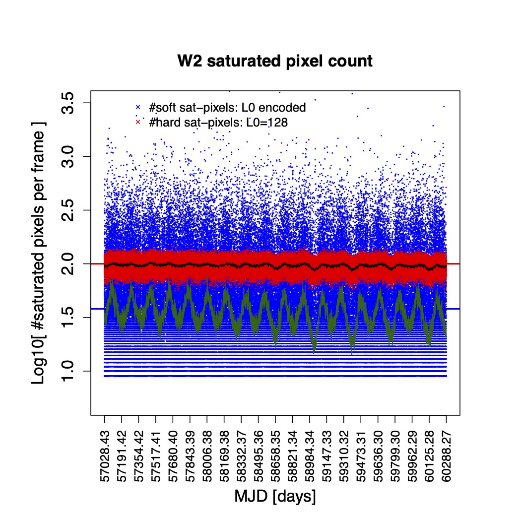Figure 6a - Number of hard (salmon) and soft (light blue) saturated pixels per array versus MJD as inferred from the on-board (DEB) encoding in Level-0 W1 frame data. Horizontal blue and red lines represent the median number of soft and hard saturated pixels respectively at the end of original post-cryo (Jan. 25 - Feb. 1, 2011). The dark blue and black curves are the 7-day wide, rolling averages for the soft and hard saturated pixel values, respectively. The green line is the temperature of the beam splitter assembly mount. Click to enlarge.	Figure 6b - Same as Figure 6a, except for W2. Click to enlarge.
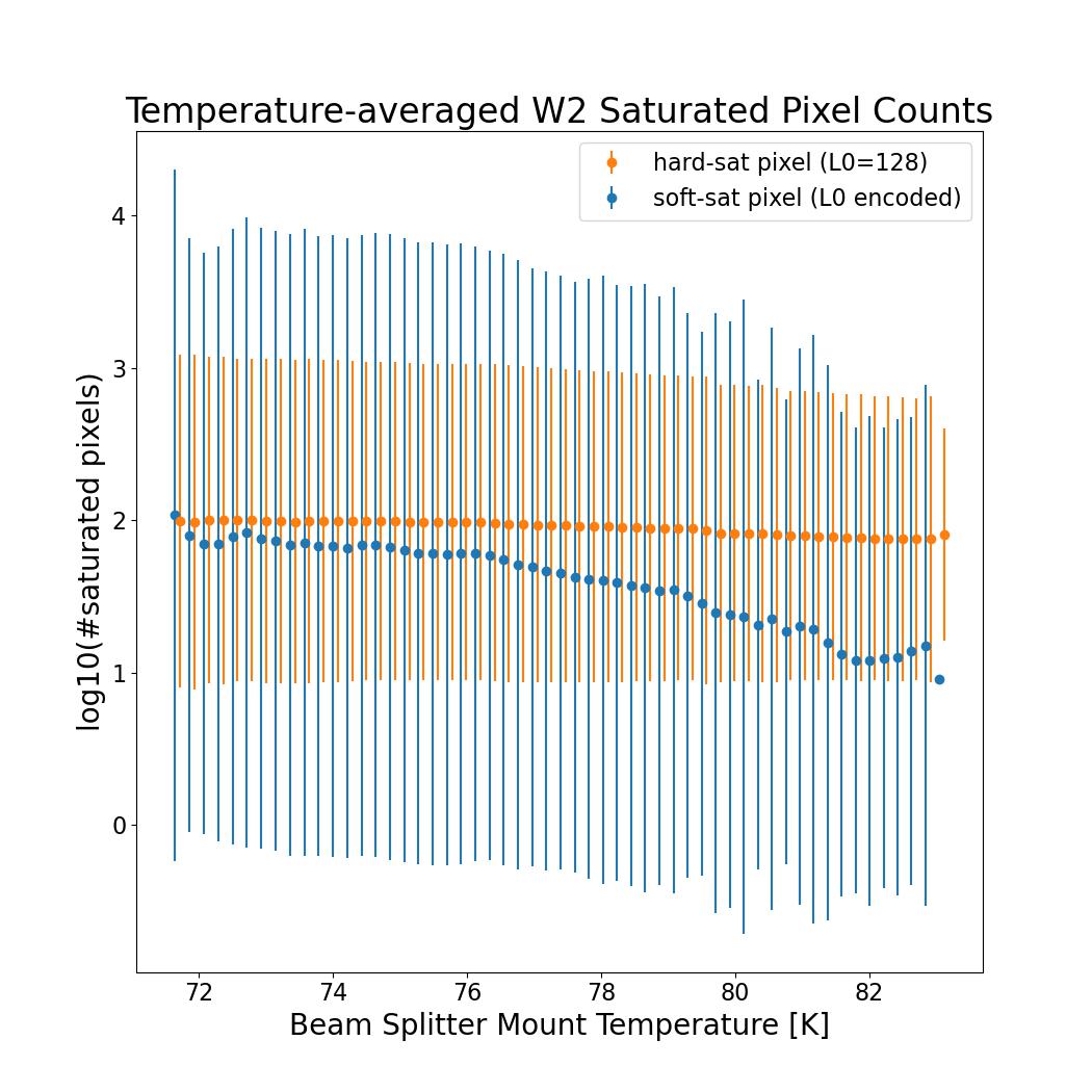Figure 6c - Number of hard and soft-saturated pixels versus beam splitter assembly mount temperature for the level-0 W1 images. The hard saturated points have been offset by +0.075 K for clarity. Click to enlarge. The data behind this figure can be found in Table 1 (.tbl file, 23 kB).	Figure 6d - Same as Figure 6c, except for W2. Click to enlarge. The data behind this figure can be found in Table 2 (.tbl file, 23 kB).

IV.2.a.iii. Bit-Mask Definitions

We made every effort to replicate the bit-mask definitions as used in earlier processing phases (4-band cryo; 3-band cryo; and 2-band post-cryo), however due to changes in detector behavior and advances in calibration methodology, there are small differences. The bit-mask definitions for the NEOWISE W1 and W2 single-exposure image masks are summarized in Table 7. As a detail, the pixels that are set to "NaN" (generally unusable) in the NEOWISE frame intensity and uncertainty products are those initially tagged with any of the following bits: 1, 3, 4, 6, 9, 10, 11, 12, 13, 14, 15, 16, 17, 18, 19 (decimal bitstring = 1048154). Furthermore, the pixels that are excluded from the profile-fit photometry measurements in the NEOWISE Source Database are those tagged with any of the following bits: 0, 1, 2, 3, 4, 5, 6, 9, 10, 11, 12, 13, 14, 15, 16, 17, 18, 19, 21, 23, 24, 27, 28, 30 (decimal bitstring = 1504706175). Note that a majority of these bits are never set in the frame masks (= "reserved" in Table 7) and are therefore meaningless. This bitstring is replicated from earlier data releases.

IV.2.a.iv. Electronic Gain, Read-Noise, and Pixel Uncertainty Estimation

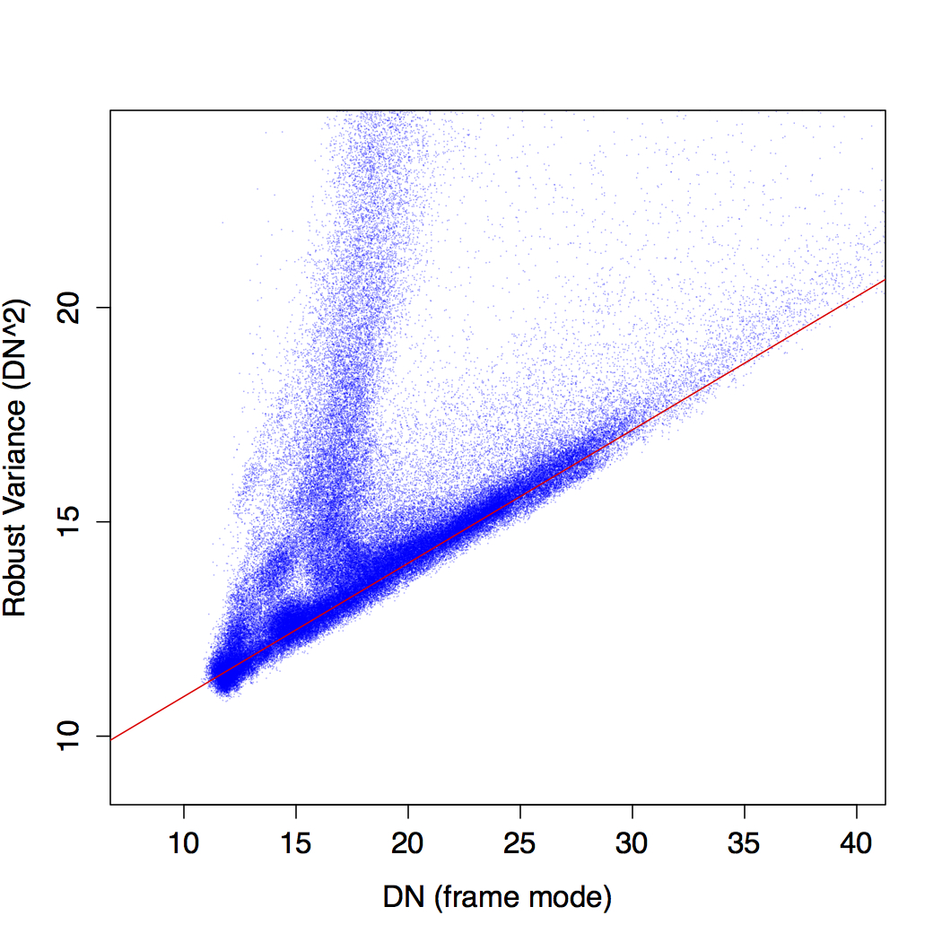
The pixel noise model is given by Eq. 2 in section IV.4.a.ii of the All-Sky Explanatory Supplement. The electronic gain and read-noise were derived in the same manner as for earlier phases of the mission (e.g., section IV.4.a.ii.1. of the All-Sky Explanatory Supplement). This entails performing a linear regression to the lower envelope of the distribution of robust frame pixel variance versus background; then estimating the electronic gain and read-noise from the fitted slope and intercept. Figure 7 shows an example of this regression using approximately 118,000 framesets towards the end of year 1 of NEOWISE.

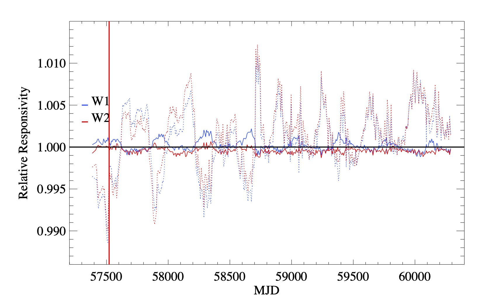
Given the large number of frames needed to robustly estimate the electronic gain and read-noise (typically two weeks' worth of data), we estimated these over-broad intervals during NEOWISE that were usually not coincident with the calibration intervals in Table 5. The trends are shown in Figures 8 and 9 and tabulated with the corresponding calibration intervals in Table 8. The trends in Figures 8 and 9 are qualitatively similar to the temperature trends in Figure 10 of section I.2.c.iii when one matches up the times at which the electronic gain and read-noise were estimated.

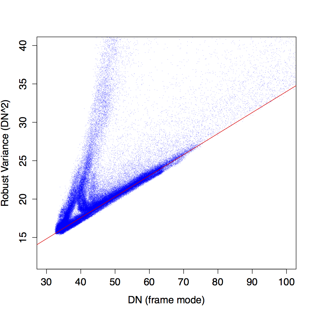Figure 7 - Robust single-exposure pixel variance versus mode using all frames in scan-range 54790a - 55289b (acquired Nov. 26 - Dec. 13, 2014). Red lines are robust linear regression fits to the lower envelope of the distributions and are used to estimate the electronic gain and read-noise. See text for details. Left: W1, right: W2. Click to enlarge.

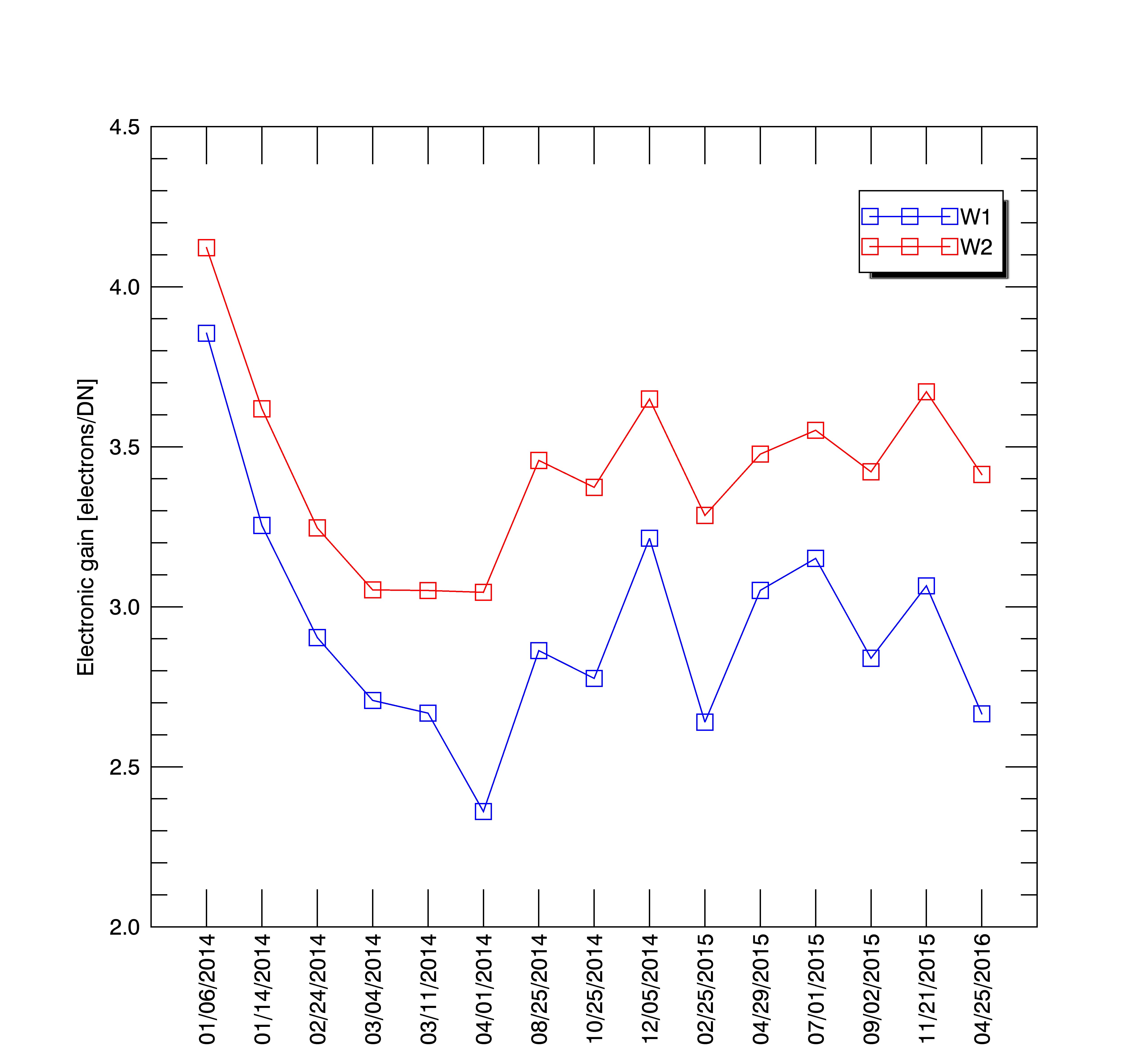Figure 8 - Electronic gain estimates as a function of date since the start of NEOWISE. Note that there have been no changes since April 2016. See text for details. Click to enlarge.

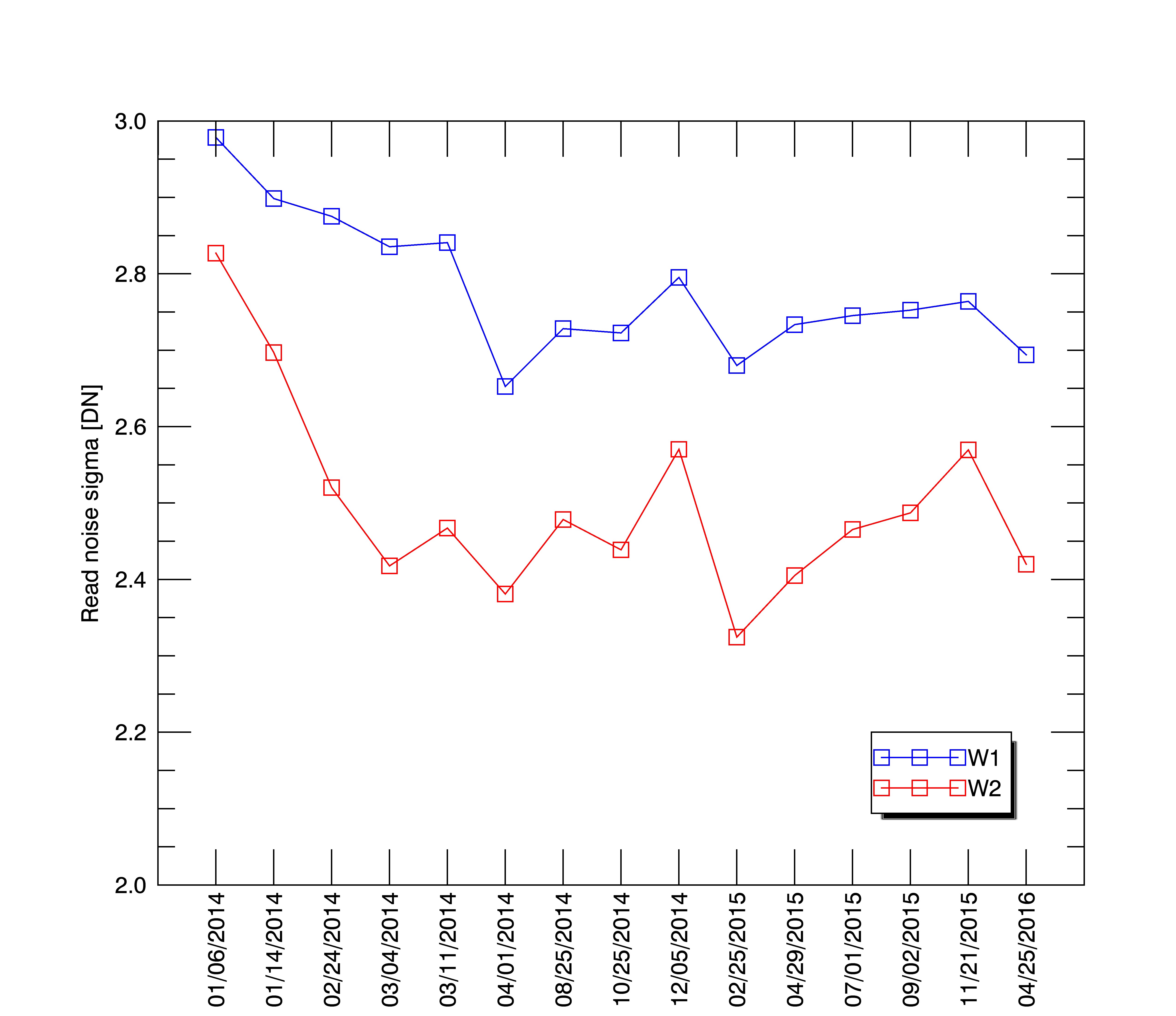Figure 9 - Read-noise sigma estimates as a function of date since the start of NEOWISE. Note that there have been no changes since April 2016. See text for details. Click to enlarge.

The read-noise sigma estimates tabulated above are single values pertaining to the entire arrays (W1 or W2). To obtain a more accurate (or representative) calibrations as a function of pixel position on each array, we used the RMS-stack maps from the temporal pixel-dispersions (step 3 in section IV.2.a.i.3) to construct effective read-noise maps. A pixel value in this read-noise map is computed using the following equation:

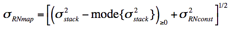(Eq. 1)

where the quantity inside the inner brackets (parenthesis) with subscript "≥0" denotes the difference between the stack-variance value for the pixel and the mode over all pixels. Differences < 0 are reset to zero and stack-variance values above the threshold used for masking noisy pixels (section IV.2.a.i.3) are reset to the threshold value itself. The last variance term in Eq. 1 is the actual read-noise variance estimate from Table 8 - a constant for each array. The read-noise map defined by Eq. 1 is used in the pixel-error model equation (Eq. 2 in section IV.4.a.ii of the All-Sky Explanatory Supplement).

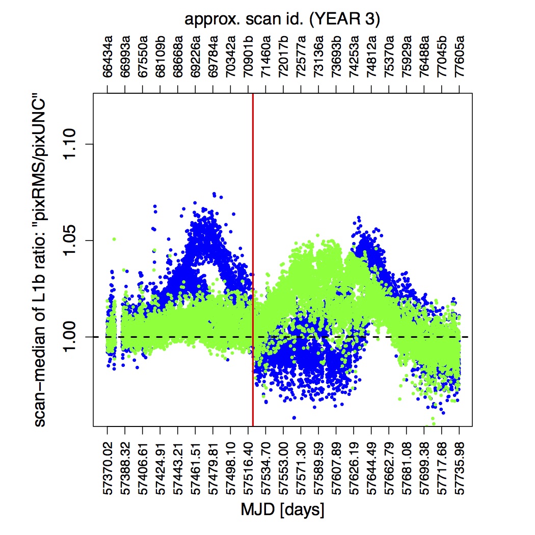
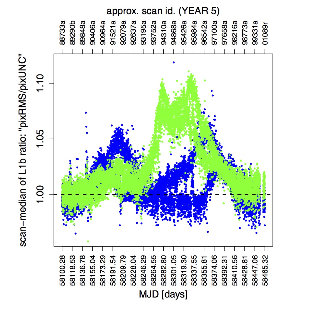
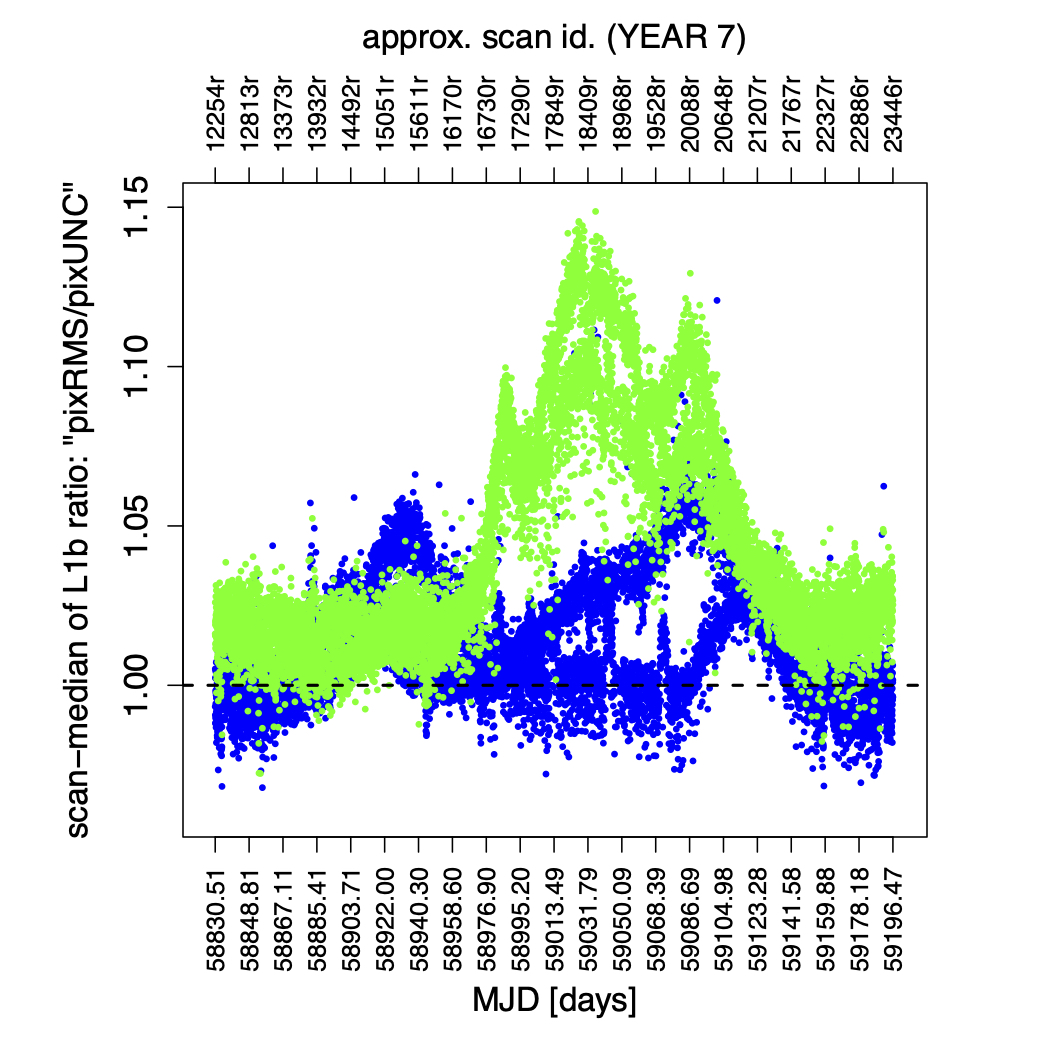
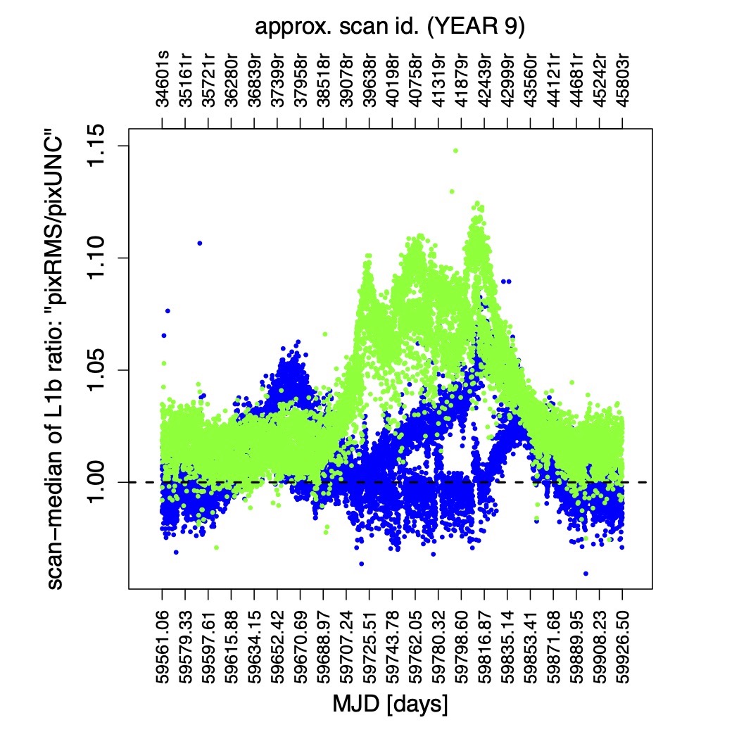
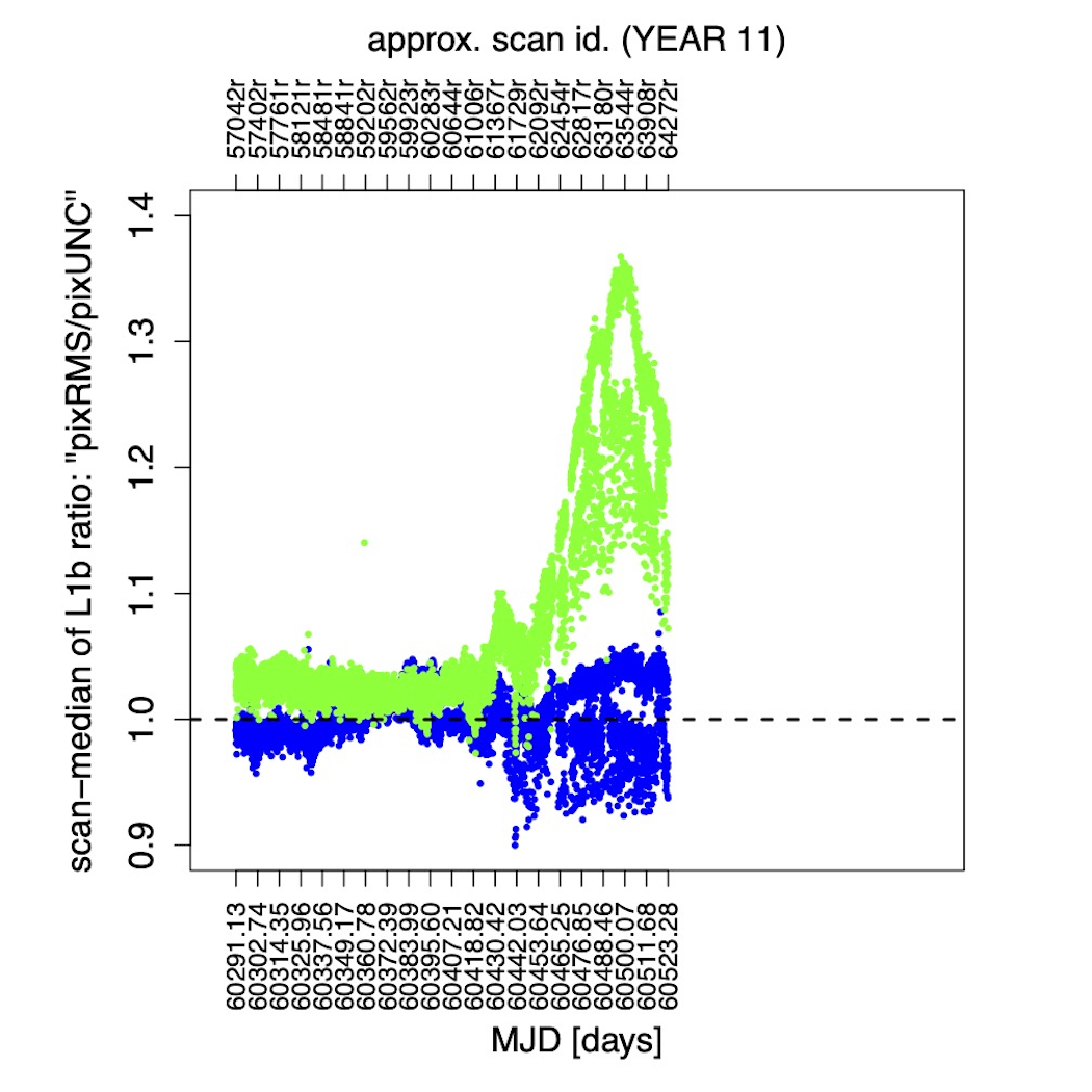
The pixel uncertainty estimates were validated against robust measurements of the RMS fluctuation about the background in the corresponding intensity frames. We used an automated algorithm to select background regions that were approximately spatially uniform and had a moderately low source density. A trimmed lower-tail standard deviation from the mode was used as a proxy for the RMS. This measure was divided by the mode of pixel uncertainties over the same regions to compute a pseudo reduced-χ metric per pixel. This measure is shown as a function of MJD in Figure 10. Apart from a few excursions (processing glitches), for W1 this metric remained mostly within 1±0.05 throughout the NEOWISE survey, implying the uncertainty model estimates tracked the noise fluctuations in pixel signals reasonably well. This is consistent with global analyses of the PSF-fit photometry to point sources where the reduced χ² values are on average ≈ 1.

The "RMS/UNC" ratios shown in Figure 10 were sometimes used to rescale the pixel-error model equation so that pixel uncertainty estimates therefrom were more-or-less consistent with local RMS values in the intensity frames. This was used for ad-hoc temporary adjustments to the error model to avoid re-deriving electronic gains, read noises, and accompanying read-noise maps since these were computationally expensive. These "RMS/UNC" ratios are what define the "uncertainty model scaling parameters" in Tables 4 and 5.

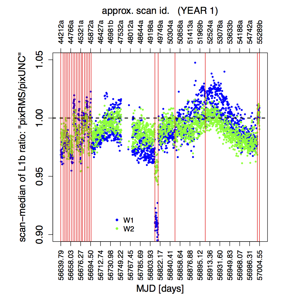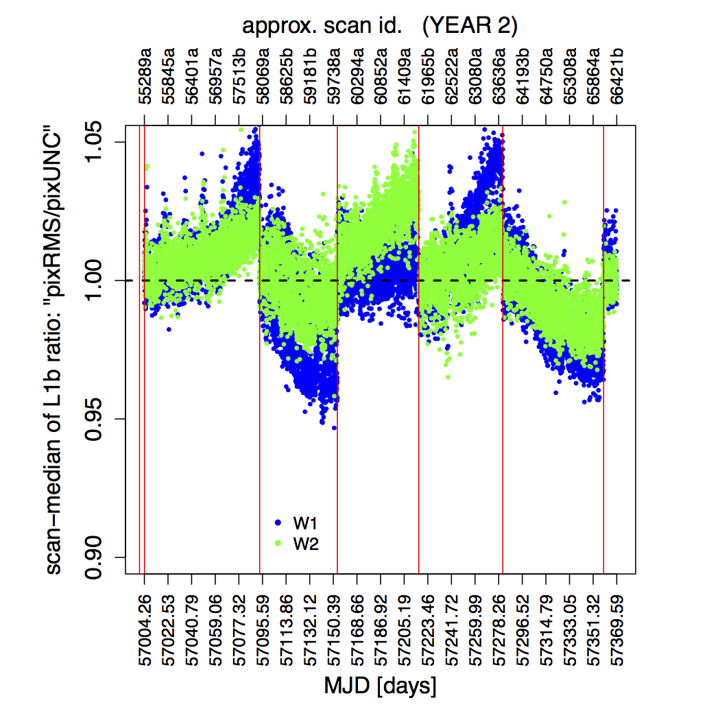Figure 10a - Medianed ratio of robust pixel RMS within specially selected frame region to mode of pixel uncertainties from noise model in the same region as a function of time over year 1 of NEOWISE. The vertical red lines mark the boundaries of the calibration intervals defined in Table 5. See text for details. Click to enlarge.	Figure 10b - Same as Figure 10a but for year 2 of NEOWISE. Click to enlarge.
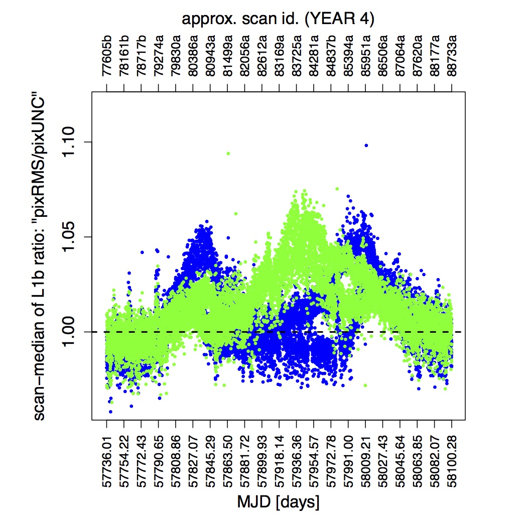Figure 10c - Same as Figure 10a but for year 3 of NEOWISE. Click to enlarge.	Figure 10d - Same as Figure 10a but for year 4 of NEOWISE. Click to enlarge.
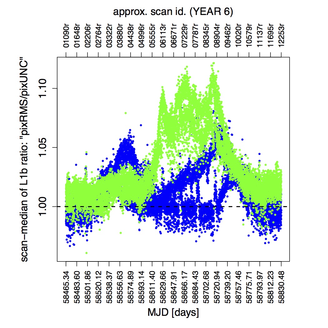Figure 10e - Same as Figure 10a but for year 5 of NEOWISE. Click to enlarge.	Figure 10f - Same as Figure 10a but for year 6 of NEOWISE. Click to enlarge.
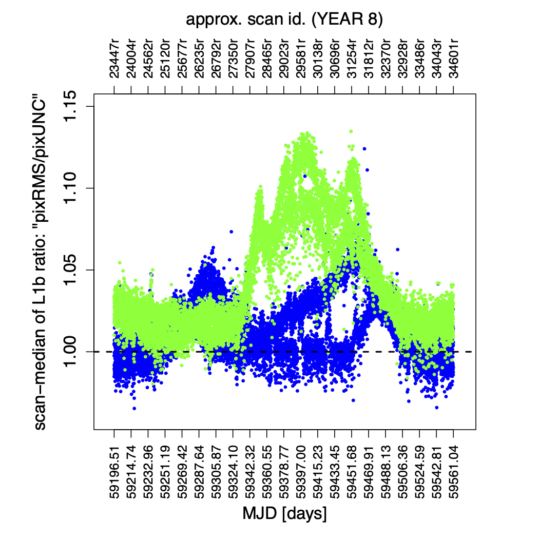Figure 10g - Same as Figure 10a but for year 7 of NEOWISE. Click to enlarge.	Figure 10h - Same as Figure 10a but for year 8 of NEOWISE. Click to enlarge.
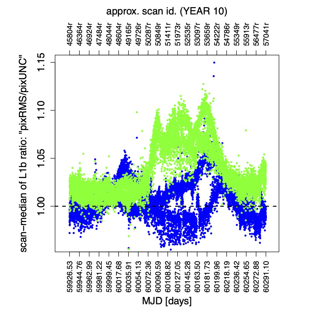Figure 10i - Same as Figure 10a but for year 9 of NEOWISE. Click to enlarge.	Figure 10j - Same as Figure 10a but for year 10 of NEOWISE. Click to enlarge.
Figure 10k - Same as Figure 10a but for year 11 of NEOWISE. Click to enlarge.

IV.2.a.v. Dark and Relative Bias Calibrations

The dark (offset) calibrations are designed to capture relative spatial variations and structure in the detector bias. They are not intended to subtract an absolute level of the dark signal. The latter is difficult since the detectors are always exposed to the sky. The dark (relative bias) maps are generated from the raw Level-0 (L0) frames by first subtracting their median-pixel signals and then stacking (collapsing) the frames using trimmed-averaging on each individual pixel. Of order 7000-9000 filtered L0 frames (per band) spanning typically four consecutive days are used when creating the darks for a specific calibration interval. By filtered, we mean omitting frames that are within 35 degrees of the moon; less than 15 degrees of the galactic plane, and within 5 degrees of the SAA boundary. Anomalously high pixel values (> 32,000 DN) are tagged in the static bad-pixel calibration masks (sections IV.2.a.i.3 and IV.2.a.ii).

Figures 11a and 11b show the dark (relative-bias) maps for W1 and W2 respectively, for three intervals during year 1 of NEOWISE. It is difficult to discern any difference by eye since the changes in the hot (hi-dark) pixel distribution over the course of the survey are only several percent (e.g., see Figure 3a). It's important to note that these dark (offset) calibrations are treated as "static" for the duration of a calibration interval and perform reasonably well at removing the cold/hot (lo/hi-dark) pixels early on. As time progresses, they become less accurate. However, this is where the dynamic sky offsets pick up the slack, i.e., help mitigate the residual lo/hi dark pixels not removed by the static darks.

Figure 11a - W1 dark (relative-bias) maps for three different periods during NEOWISE: Dec. 15, 2013 (left); June 14, 2014 (middle); Dec. 10, 2014 (right). Click to enlarge.

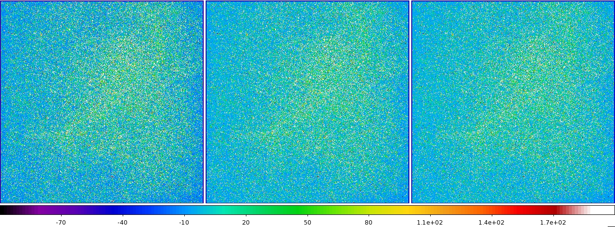Figure 11b - W2 dark (relative-bias) maps for three different periods during NEOWISE: Dec. 15, 2013 (left); June 14, 2014 (middle); Dec. 10, 2014 (right). Click to enlarge.

IV.2.a.vi. Channel-noise Corrections

An overview of the "basics" of the channel-noise correction algorithm as used to process frames for the All-Sky and 3-band Cryo Data Releases is given in section IV.4.a. of the All-Sky Explanatory Supplement. There we made extensive use of the "reference" pixels at the ends of each amplifier channel, i.e., which mostly contained the respective bias levels that correlated well with signals in the active regions of each channel. However, as we progressed into the post-cryo phase (including reactivation in late 2013), the reference pixels did not perform as well at predicting the underlying bias levels. We resorted to correct for the "bulk channel fluctuations" using the active pixels for each channel. This entailed computing the pixel mode in each channel and checking for significant offsets relative to the adjacent channels. If significant, the levels were then equalized across channels. We further improved the robustness of the algorithm following reactivation. This involved first regularizing an input frame by estimating and subtracting a robust Slowly Varying Background (SVB) and resetting high signals greater than some threshold to 0. This created an internal working image from which the channel corrections could be robustly estimated. These corrections were then applied to the original input frame. All parameters (20 in total per band) were re-tuned for NEOWISE. Figure 12 shows a blink animation of a W2 NEOWISE frame processed with and without the new channel-noise correction algorithm.

Figure 12 - Click for a blink-animation of a W2 frame processed with and without the new channel-noise correction algorithm optimized for NEOWISE (internal WSDS software delivery version 7.5).

The channel-noise correction algorithm performed extraordinarily well for NEOWISE, or at least much better than it did for the earlier processing phases. However, one rare (small) caveat remains for NEOWISE. Occasionally, when the detectors observed a large background gradient perpendicular to the detector read-out (amplifier) channels, the channel-noise correction algorithm could not reliably correct for the intrinsic channel-to-channel variations, resulting in very large residual gradients. This effect was most common in W1 due to its greater sensitivity to background gradients relative to the underlying ambient and zodiacal backgrounds, particularly when a bright off-axis source perpendicular to the scan direction was present since the W1 detector channels are aligned with the scan direction. There was a small update to the algorithm (a threshold parameter) on 5/20/2014 to mitigate this effect.

IV.2.a.vii. Linearity Calibration

We retained the same non-linearity calibration as was derived from ground test data and used to correct the 4-band, 3-band cryo, and 2-band post-cryo data in earlier processing phases. The formalism was described in detail in section IV.4.a.vi of the All-Sky Explanatory Supplement. The relevant correction formulae (per pixel) are given by Equations (18) and (20) therein.

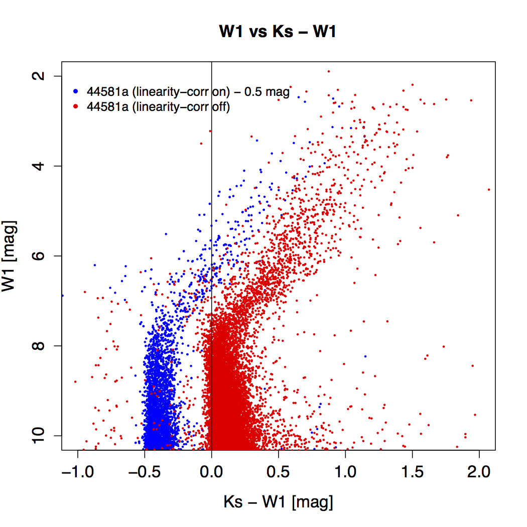
It was very difficult to validate the accuracy of the non-linearity calibration for the W1, W2 NEOWISE frames. Our best diagnostic was from examining color-magnitude diagrams and looking for systematic deviations in the trends expected for known stellar populations. One complicating issue is the presence of a bias in the PSF-fit photometry of saturated sources in W1 and W2. Figure 13 shows examples of color-magnitude diagrams involving the 2MASS K_s band. Instead of classically narrow (and vertical) color distributions, these turn "wild" at magnitudes brighter than W1 ~ 8 and W2 ~ 7 (the approximate saturation limits). At first, we thought an erroneous non-linearity correction was to blame, but this does not appear to be the case. Turning off the non-linearity correction makes little difference, in fact, it leads to an increased scatter (red points) in the photometry. Furthermore, the behavior for saturated sources is such that their estimated fluxes become relatively brighter the brighter they are. If due to non-linearity, it would require a correction that reduces flux for bright sources. At the time of writing, this does not conform with the traditional behavior of MgCdTe detectors as characterized in the laboratory and on other facilities.

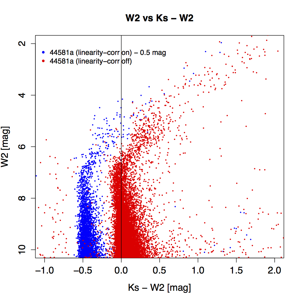Figure 13 - Color-magnitude diagrams involving the 2MASS Ks band to explore the impact of the linearity corrections (on versus off). Detector non-linearity cannot explain the growing bias for fluxes brighter than the W1 and W2 saturation limits (~ 8 and ~ 7 mag. respectively). All NEOWISE photometry is PSF-fit photometry from the single-exposure source database. See text for details. Left: W1, right: W2. Click to enlarge.

IV.2.a.viii. Relative Responsivity (Flat-field) Calibrations

The high-spatial frequency (pixel-to-pixel) relative responsivity maps (or flat fields) were generated from the raw Level-0 (L0) frames using the "change-in-background" method. Here, we measure the change in intensity in a pixel (i.e., slope) in response to the variation in overall intensity on a frame as the astrophysical (e.g., zodiacal) background varies. For details see section IV.4.a.v of the All-Sky Explanatory Supplement. This "change-in-background" method helped mitigate incomplete knowledge of the absolute instrumental dark/bias level.

Of order 7000-9000 filtered L0 frames (per band) spanning typically four consecutive days are used when creating flat-fields for a specific calibration interval. This number was sufficient to fill the detector wells and obtain good signal-to-noise per pixel (typically 50 or more). By filtered, we mean omitting frames that are within 35 degrees of the moon; less than 15 degrees of the galactic plane, and within 5 degrees of the SAA boundary. Anomalously low/high relative responsivity values (< 0.1 / > 1.8) are reset to unity and tagged in the static bad-pixel calibration masks (sections IV.2.a.i.3 and IV.2.a.ii).

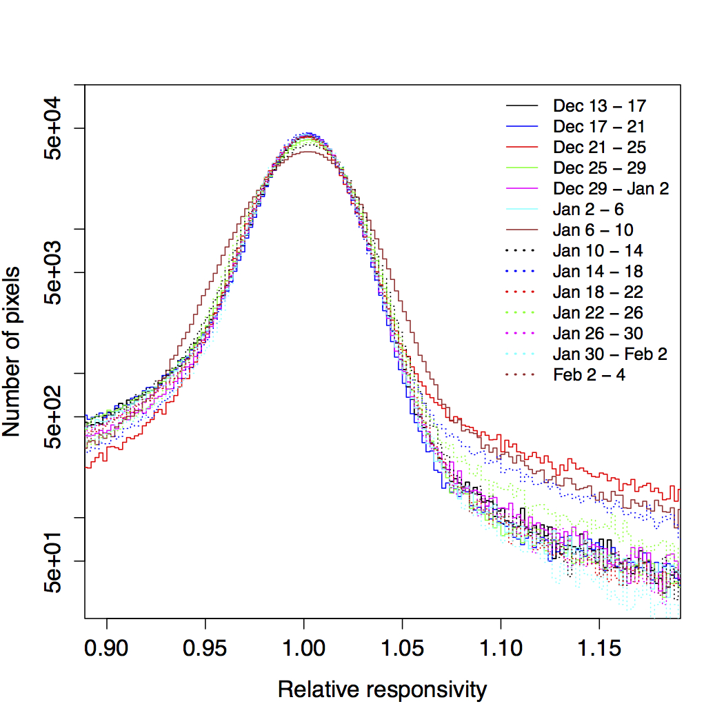
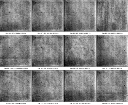
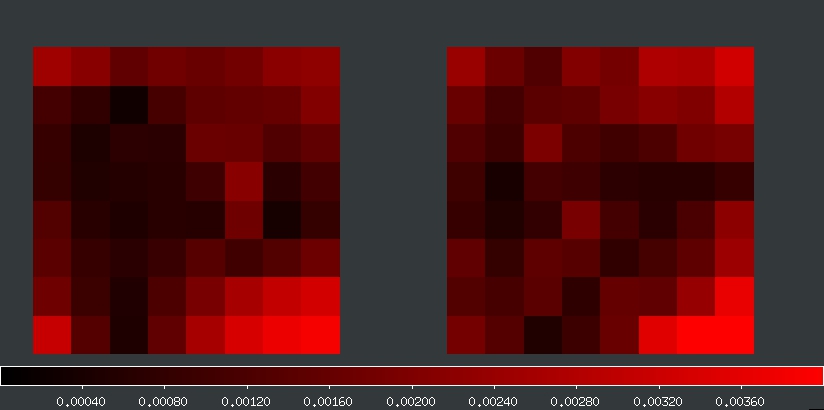
Due to the rapid cooling following reactivation, more (narrower) calibration time intervals were used early in the NEOWISE survey. Histograms of the derived relative-responsivity for the W1 and W2 arrays during this period are shown in Figure 14. Most of the variation during this period occurred for pixels in the high responsivity tail. The overall responsivity pattern on each array then stabilized around mid-February 2014. All the W1,W2 responsivity maps made during the first year of the NEOWISE survey are shown in Figures 15 and 16. Most of these were made for spot-checks and regular instrumental trending, but some (where pertinent) were used to construct new calibration intervals (e.g., see update history in Table 5).

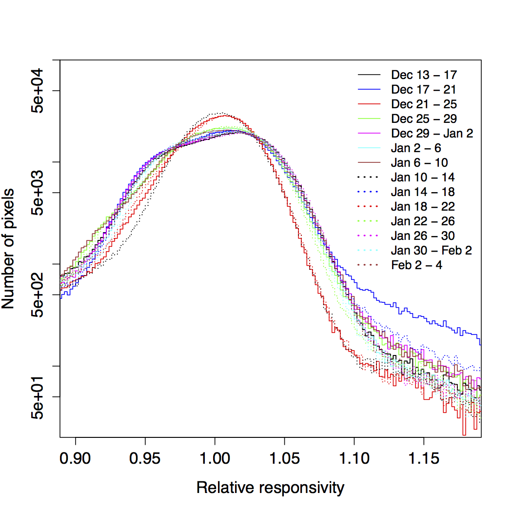Figure 14 - Histograms of the relative pixel-to-pixel responsivity as a function of date during the early cool-down period following reactivation of the detectors. See text for details. Left: W1, right: W2. Click to enlarge.

Figure 15 - Click to view a PDF file of all the W1 relative-responsivity calibration maps made during year 1 of NEOWISE. Image stretch is 0.97 (darkest) to 1.03 (brightest) in all maps.	Figure 16 - Click to view a PDF file of all the W2 relative-responsivity calibration maps made during year 1 of NEOWISE. Image stretch is 0.97 (darkest) to 1.03 (brightest) in all maps.

IV.2.a.viii.1. Performance of Responsivity Calibrations

To validate the performance of our relative spatial responsivity corrections in general, we periodically analyzed the source photometry from ~200 scans, or ~45,000 frames after filtering to avoid contamination from the moon, galactic plane, and/or SAA. The NEOWISE-extracted sources were then spatially binned and their photometry differenced with the photometry of matching sources in the AllWISE Data Release Catalog. This catalog was generated from co-adding (averaging) many dithered exposures and is thus expected to be immune to residual patterns in the relative responsivity on the scale of individual exposures. It, therefore, provides a good reference catalog. The NEOWISE - AllWISE photometric difference maps are then normalized and smoothed using a constant Gaussian kernel to remove the binning pattern and yield the low-spatial frequency relative responsivity maps.

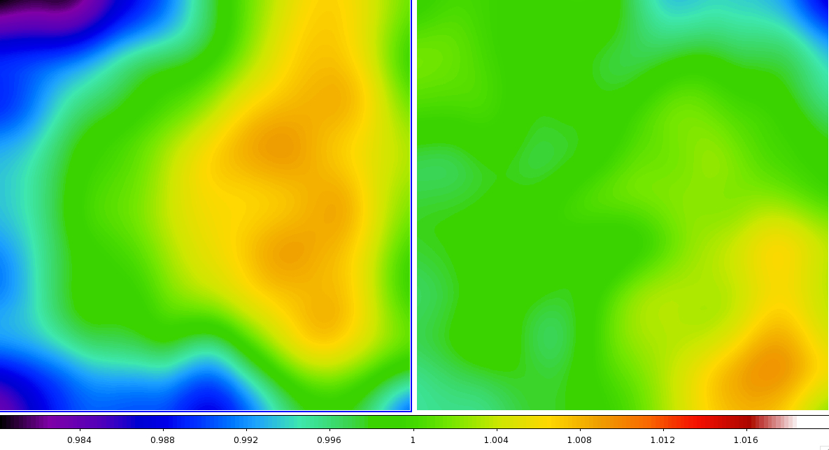
If our relative responsivity corrections were perfect (to their achievable accuracy), the low-spatial frequency residuals should be close to unity everywhere. Figure 17 shows some typical low-spatial frequency residual responsivity maps we obtained during year 1 of NEOWISE. The bulk of the residuals are within 1±0.016 (or ±1.6%) for W1 and slightly less for W2. At times, they may have been as high as ±4%. Therefore, repeated single-exposure photometry across multiple exposures covering the same sky region is likely to show the same scatter.

Figure 17 - Residual low spatial-frequency responsivity maps created from stack-averaging spatially binned "NEOWISE - AllWISE" photometry differences using sources extracted from > 45,000 single-exposure frames acquired over one period in year 1 of NEOWISE. The color bars denote the relative size of the residuals. See text for details. Left: W1, right: W2. Click to enlarge.

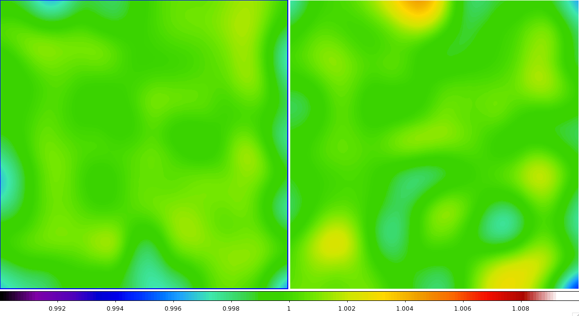
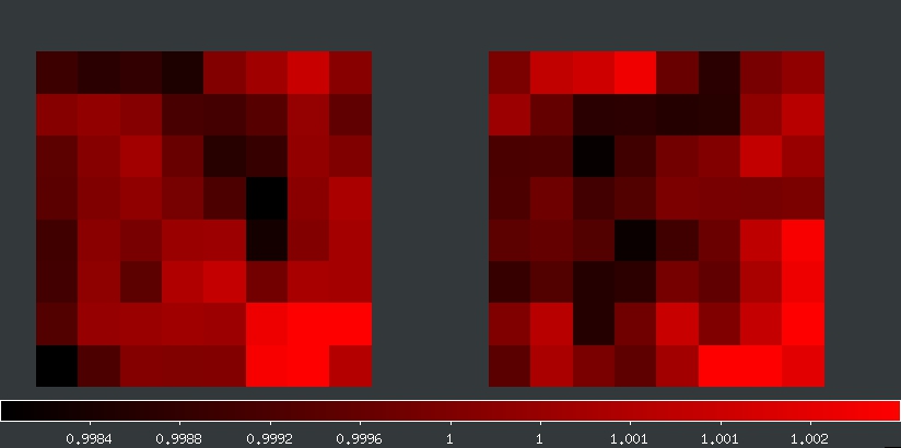
The cause of these residuals could not be resolved for most of year 1 of NEOWISE. It appeared that the high-spatial frequency (pixel-to-pixel) relative responsivity maps described in section IV.2.a.viii could not capture throughput variations at low-spatial frequencies, perhaps induced by non-uniformities in the optical train. Towards the end of year 1 however, we decided to adopt a two-step calibration process whereby we augmented the high-spatial frequency maps by multiplying them with the low-frequency maps (using spatially-binned differenced photometry from a first processing pass) and renormalizing to create new effective flat-field calibrations. Figure 18 shows an example of the residuals following this augmentation for data processed early in year 2 of NEOWISE. The improvement is dramatic. The low-spatial frequency residuals in the single-exposure products are suppressed to better than ±0.6%. This method was used for the remainder of the NEOWISE survey.

Figure 18 - Residual low spatial-frequency responsivity maps created from stack-averaging spatially binned "NEOWISE - AllWISE" photometry differences using sources extracted from > 45,000 single-exposure frames acquired over one period immediately after year 1 of NEOWISE (i.e., into year 2). To be compared with Figure 17. The color bars denote the relative size of the residuals. See text for details. Left: W1, right: W2. Click to enlarge.

IV.2.a.viii.2. Responsivity Trending

Responsivity maps such as those in Figure 18 are now generated on a weekly basis to keep track of the positions and magnitudes of variations and to determine when calibration updates may become necessary. Figure 18a shows both the RMS and the minimum and maximum values of the relative responsivity during years 3 through 11 of NEOWISE. All quantities (min, max, RMS) are highly correlated between W1 and W2, indicating that the variations are due to optical effects and are generated upstream of the W1/W2 dichroic.

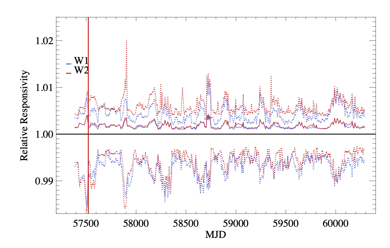Figure 18a - RMS, minimum, and maximum responsivities measured over years 3 through 11 of NEOWISE from weekly responsivity maps such as Figure 18. RMS + 1.0 for W1 and W2 are shown by the solid lines, while the maximum and minimum responsivities are shown as dotted lines. The last recalibration from Table 5 is indicated by the vertical red line. Click to enlarge.

The magnitudes of the variations in responsivity depend strongly on the position in the focal plane. Figure 18b shows the RMS in responsivity over time in blocks of 128 x 128 pixels. Both W1 and W2 show a similar pattern, with relatively stable regions to the left of array center (where sigma ≈ 0.0005), and more strongly-varying regions at the corners of the arrays. The upper-right and lower-right corners are particularly volatile, with 1-sigma variations more than eight times larger. The responsivity variations in these regions over time are compared in Figure 18c. The relative responsivities show a clear annual periodicity, though the sense of the variations may be out of phase from one part of the array to another. Moreover, in the least stable parts of the arrays the relative responsivities can vary by more than 1% over a span of less than two months. It is neither desirable nor practical to recalibrate the photometry pipeline on such short time scales, and the responsivity variations will obviously contribute to the photometric noise floor. On longer time scales, averaging over the relative responsitivities (Figure 18d) shows there is very little bias from one part of the array to another, with sigma < 0.1% and the worst outliers at ≈ 0.2%.

Figure 18b - RMS in the responsivity variations over time in 128 x 128 pixel blocks in W1 (left) and W2 (right). The stretch extends linearly from 0 to 0.004, and pixels in the lower-right corners have sigma = 0.004.

Figure 18c - Variations in responsivity over years 3 through 11 of NEOWISE of pixels with 129 < x < 256, 384 < y < 512 (solid lines) and 896 < x < 1024, 1 < y < 128 (dotted lines). The last recalibration from Table 5) is indicated by the vertical red line. Click to enlarge.

Figure 18d - Mean relative responsivities, averaged over years 3 through 11, in 128 x 128 pixel blocks in W1 (left) and W2 (right). The stretch extends linearly from 0.998 to 1.003.

IV.2.a.ix. Dynamic Calibrations

The purpose of dynamic calibration (dynacal) is to capture instrumental variations and transients as close as possible to the frame observation time and then correct them. NEOWISE processing used the same dynacal methodology as in 4-band cryo for W1 and W2, as outlined in section IV.4.a.viii of the All-Sky Explanatory Supplement. Two dynamic calibrations are performed for NEOWISE: (i) sky offsets and (ii) the detection and tagging of temporal bad-pixel transients.

The sky offsets are computed using a single frame-step moving median along a scan of pre-calibrated frames that are dark subtracted, linearized, and flattened using "static" calibrations (see intervals in Table 5). The frame median is subtracted from each frame prior to median combining and frames contaminated by an excess of cosmic rays or with a high source density (e.g., close to the galactic plane) are omitted. Note that the actual frame where the sky offset is applied (subtracted) is omitted from the window on which the moving median is computed. This is to avoid "incestuously calibrating" a frame using information about itself (e.g., see the "histogram-spike anomaly" reported in early processing phases). The moving median is 37 frames long with a minimum of 29. Below this minimum, dynacal assigns the best calibration product closest in time to the frame in question. Frames at the start or end of a scan boundary (or within half a window length from a boundary) are assigned an "inner" sky-offset product that's closest in time.

The sky-offset products are intended to capture and correct spatial variations in the relative dark/bias level over frames, including cold and hot pixels not removed by the static dark (relative bias) maps (section IV.2.a.v). I.e., as a static dark loses its accuracy over time, the sky offset can still correct the spatial variations. This can be seen in Figures 19 and 20. These show the trend in the number of low/high-tail pixels in the sky-offset histograms (below/above thresholds of -20/+20 DN). Close to the start of a calibration interval (red vertical lines), the number of low/high-tail pixels is generally low since the static dark subtracts them reasonably well, however, late in an interval, the numbers can be high since the static dark is out of synch with the true state of the detector. The variation within an interval is also influenced by seasonal temperature changes (e.g., Figure 3a).

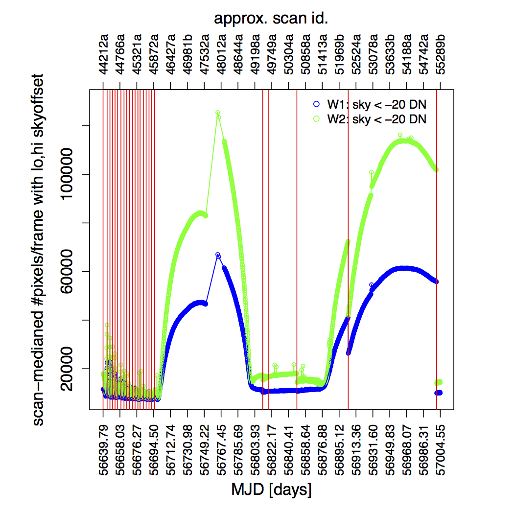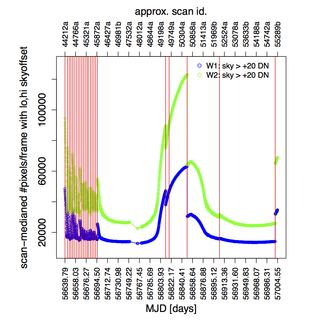Figure 19 - Number of pixels in low tails (< -20 DN) of sky-offset pixel distributions (medianed over all frames per scan) as a function of time over year 1 of NEOWISE. The vertical red lines mark the boundaries of the calibration intervals defined in Table 5. See text for details. Click to enlarge.	Figure 20 - Number of pixels in high tails (> +20 DN) of sky-offset pixel distributions (medianed over all frames per scan) as a function of time over year 1 of NEOWISE. The vertical red lines mark the boundaries of the calibration intervals defined in Table 5. See text for details. Click to enlarge.

The second type of dynamic processing in ICal is the detection and tagging of temporal bad-pixel transients (bit #21 in Table 4). The intent here is to tag spatial outliers (low/high pixel spikes) that persist for N consecutive frames for the same pixel along a scan. The method is described in section IV.4.a.viii.3 of the All-Sky Explanatory Supplement. For NEOWISE, we assumed N = 5. This operation, therefore, combines both the spatial and temporal dimensions and excludes pixels that were already tagged by the static mask bits (bits 0...7 in Table 7). It is performed before the final detection and replacement of spatial outliers (glitches) described in section IV.2.a.x. The tagging of persistent transients is therefore somewhat redundant but conservative, i.e., it provides additional protection against outliers that escape removal by the dynamic sky offsets.

IV.2.a.x. Spatial-outlier (Glitch) Replacement and Masking

The detection of spatial outliers (low/high pixel spikes) relative to the local background level is accomplished using the same median-filtering approach as used in earlier processing phases, e.g., see section IV.4.a.ix of the All-Sky Explanatory Supplement. This is performed at the end of processing in the ICal pipeline but prior to setting "fatally-bad" pixels to NaNs. If an outlier spike (either low or high) is found, mask bit #28 is set in the accompanying frame mask (section IV.2.a.iii). These pixels are not declared unusable (i.e., "fatal") and hence are not NaN'd.

An additional detail for NEOWISE single-exposure processing is that every spatial outlier that's tagged in the mask is replaced in the intensity frames with a median of its neighboring pixels. Note that there's logic to avoid replacing spikes near/on real source signal. This is to avoid biasing source flux by inadvertently clipping the cores of bright sources. Therefore, given this replacement, a pixel tagged as a spatial outlier (bit #28) in the frame mask will not mean that you will see an outlier at this position in the intensity frame, however, you have the option of omitting this pixel from your analysis if the actual replacement was not optimal.

xi. Generic Pixel-Calibration Performance

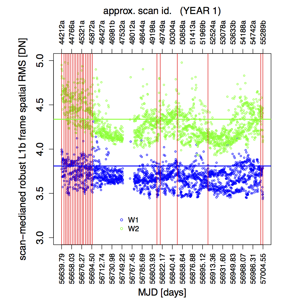
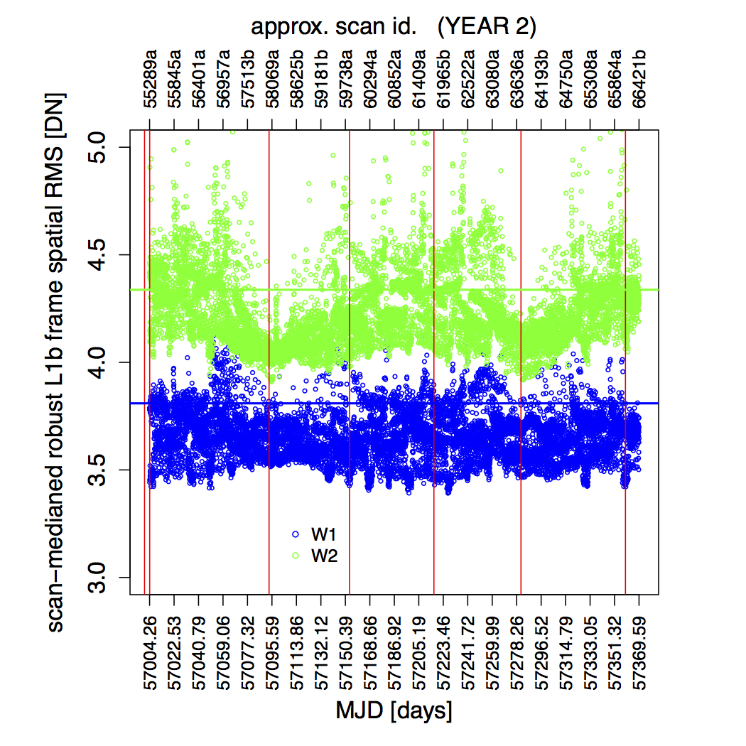
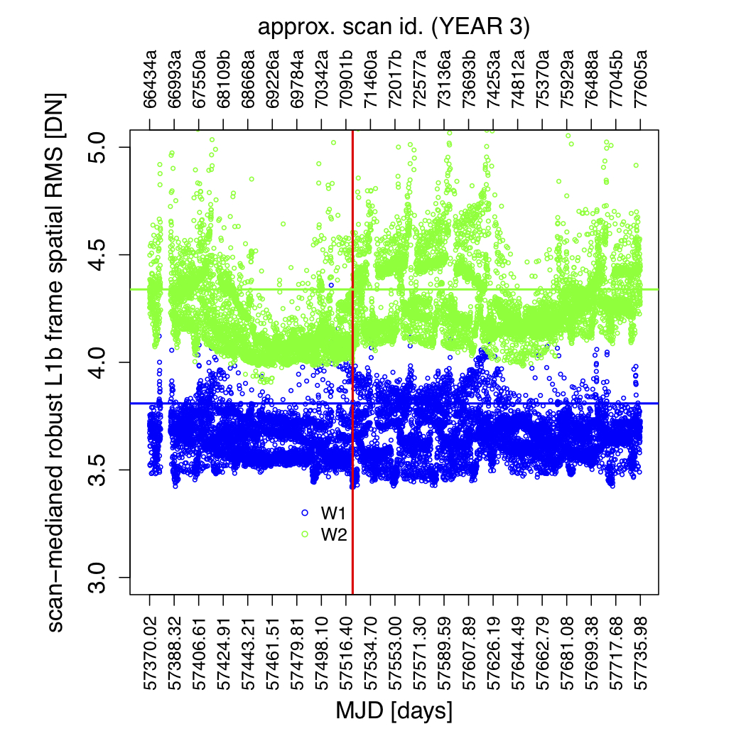
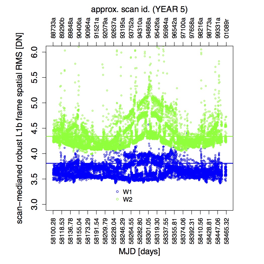
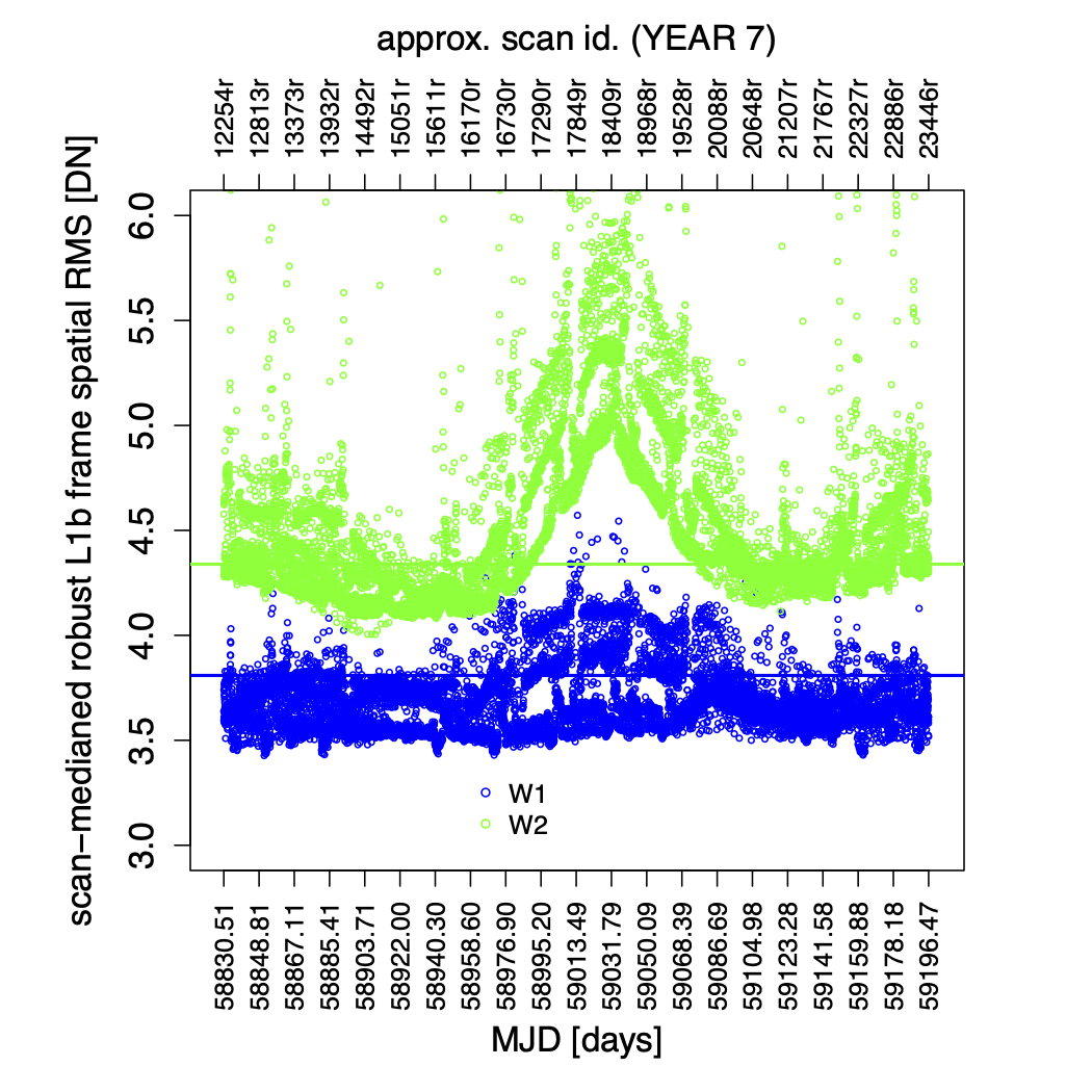
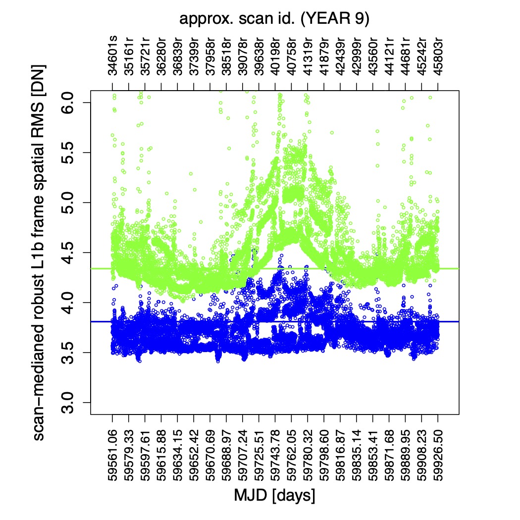
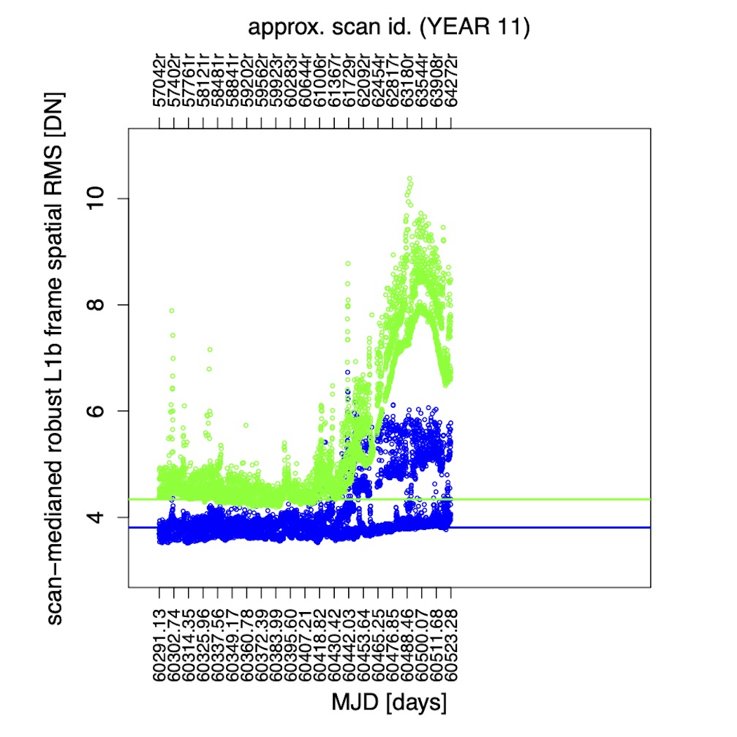
To explore our overall instrumental calibration performance, we computed a robust measure of the pixel RMS per frame based on percentile differences and then computed a global median over all filtered frames per scan. The filtering avoided frames contaminated by the moon, galactic plane, and/or SAA. This scan-medianed RMS is shown as a function of MJD in Figure 21. Its intent is to infer the relative calibration performance throughout the NEOWISE survey. Also, it is worth noting that the pixel RMS in the NEOWISE single-exposure products is lower in general than the median values from the last week of the original post-cryo phase (Jan. 25–Feb. 1, 2011), i.e., the horizontal lines in Figure 21.

Figure 21a - Robust pixel RMS medianed over all calibrated frames per scan as a function of time over year 1 of NEOWISE. The vertical red lines mark the boundaries of the calibration intervals defined in Table 5. The horizontal blue and green lines (W1 and W2 respectively) are the median RMS values from the last week of original post-cryo (Jan. 25–Feb. 1, 2011). Click to enlarge.	Figure 21b - Same as Figure 21a but for year 2 of NEOWISE. Click to enlarge.
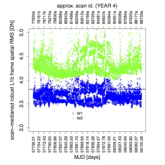Figure 21c - Same as Figure 21a but for year 3 of NEOWISE. Click to enlarge.	Figure 21d - Same as Figure 21a but for year 4 of NEOWISE. Click to enlarge.
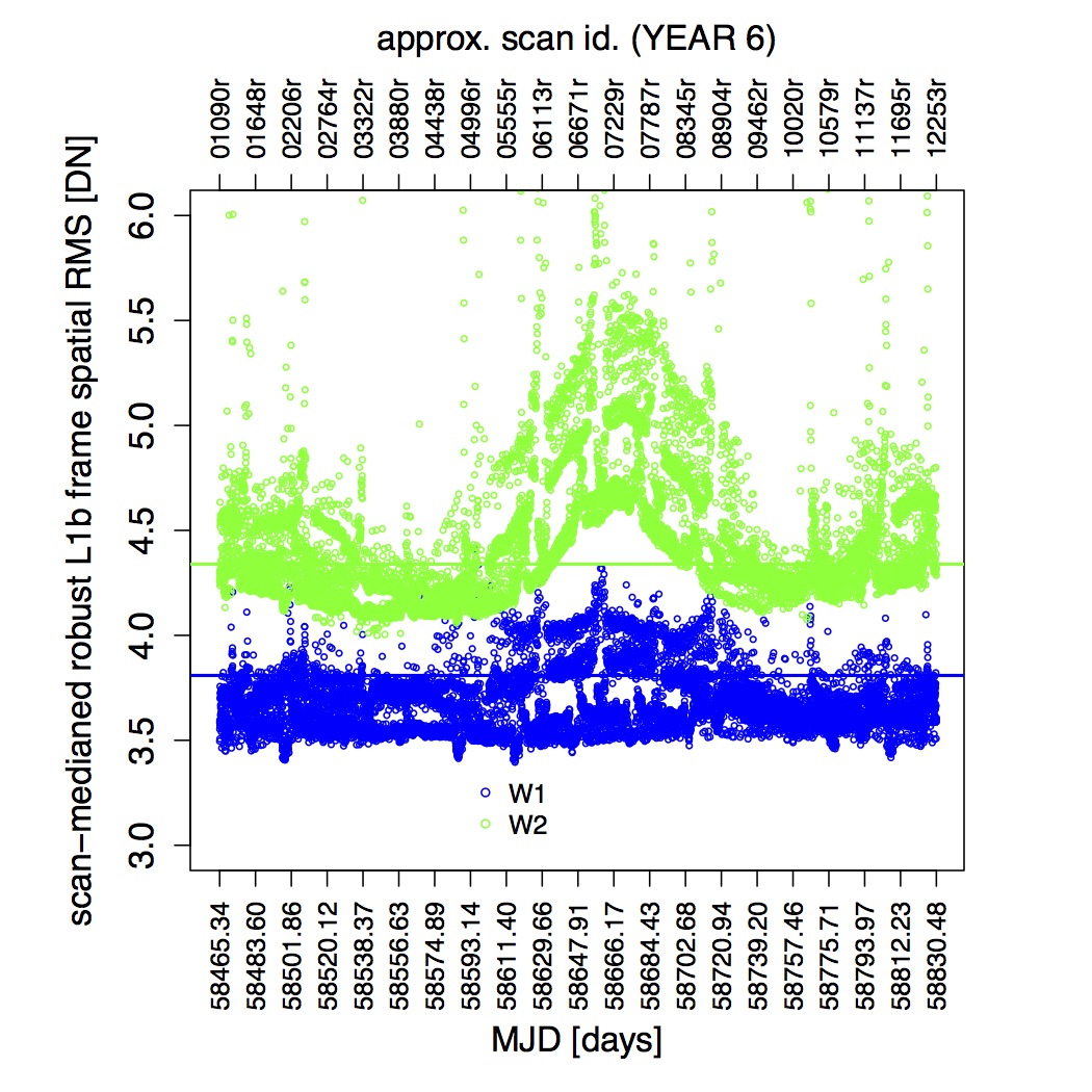Figure 21e - Same as Figure 21a but for year 5 of NEOWISE. Note the change in scale from years 1-4. Click to enlarge.	Figure 21f - Same as Figure 21a but for year 6 of NEOWISE. Note the change in scale from years 1-4. Click to enlarge.
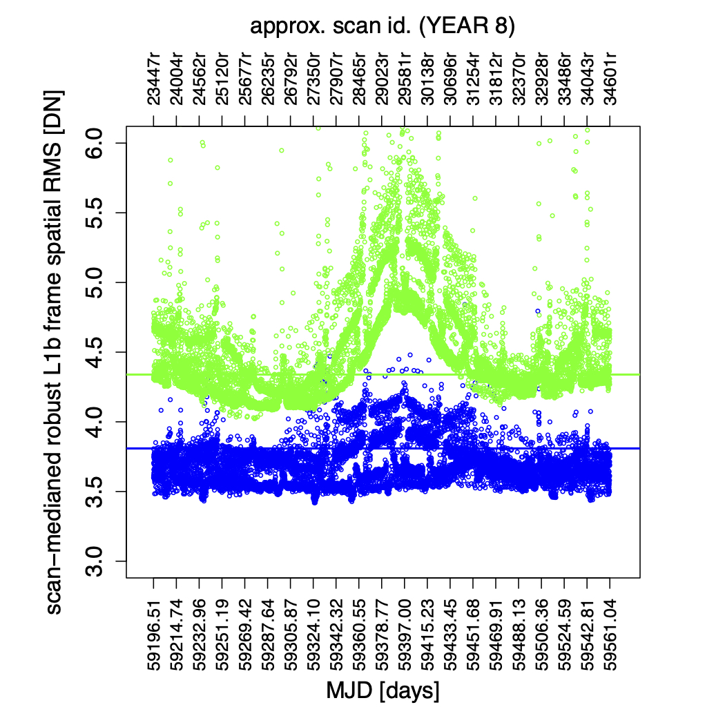Figure 21g - Same as Figure 21a but for year 7 of NEOWISE. Note the change in scale from years 1-4. Click to enlarge.	Figure 21h - Same as Figure 21a but for year 8 of NEOWISE. Note the change in scale from years 1-4. Click to enlarge.
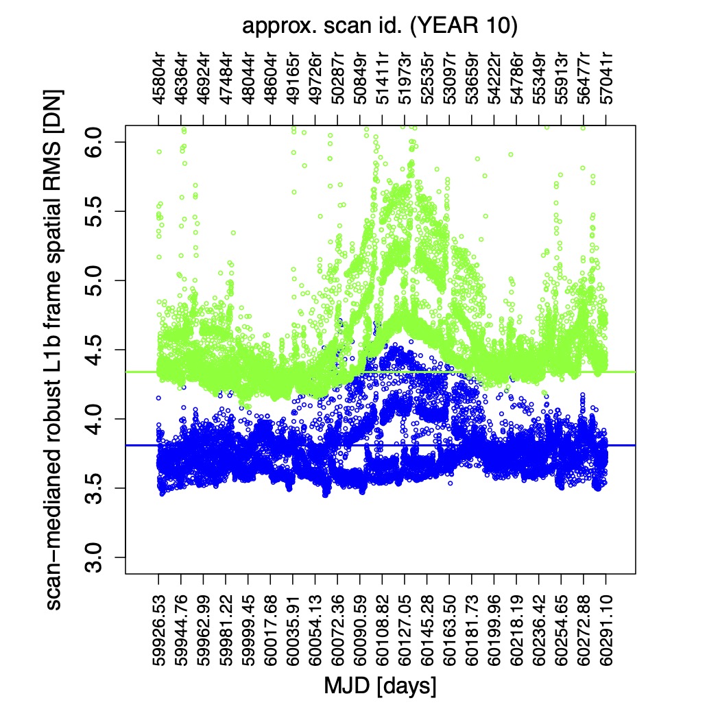Figure 21i - Same as Figure 21a but for year 9 of NEOWISE. Note the change in scale from years 1-4. Click to enlarge.	Figure 21j - Same as Figure 21a but for year 10 of NEOWISE. Note the change in scale from years 1-4. Click to enlarge.
Figure 21k - Same as Figure 21a but for year 11 of NEOWISE. Note the large change in scale from years 1-4. Click to enlarge.

Last update: 12 November 2024