VII. 3-Band Cryo Data Release

3. 3-Band Cryo Data Processing

b. Single Frame Exposure Instrumental Calibration (ICal)

Contents

i. Overview

The instrumental calibration (ICal) of single-exposure frames from the 4-band (All-Sky) cryogenic phase of the mission was described in section IV.4.a. We outline below the updates made to support ICal processing of the 3-band cryogenic single-exposure data (acquired ~ Aug 6 - Sep 29, 2010). The primary difference here is the use of time-dependent calibrations for all bands (w1, w2, w3). We also expand on some instrumental signatures and anomalies in the products that could not be accurately corrected in processing. The processing flow (per exposure) is essentially the same as that shown in Figure 1 of section IV.4.a.

i.1. Calibration Summary

The pertinent detector calibrations are summarized in Table 1. Also shown is the origin of the data used to derive the calibration product for each band ("ground", In-Orbit Checkout [IOC], "3 or 4-band survey"), and whether the calibration is time(t)-dependent, static, or dynamic throughout the 3-band cryo phase. Note that "time-dependent" is not the same as "dynamic". Time-dependent refers to calibrations that are unique to a specific (usually broad) time-span (see Table 2), while "dynamic" refers to on-the-fly flight-derived calibrations made a per-frame basis: i.e., delta-flats, sky-offsets, and transient bad-pixel tagging (section VII.3.b.viii).

Table 2 shows the scan-frame ID ranges that define the time-dependent calibration periods. Also shown are calibrated values of the electronic gain and read-noise sigma used to estimate pixel uncertainties via the error model. These are further discussed in section VII.3.b.iii.

1. The exposure time for W1 and W2 remained fixed at the nominal 7.7 seconds throughout the 3-band cryo period.
2. Derivation of the electronic gains and read-noise sigmas is discussed in section VII.3.b.iii.
3. The W3 electronic gain and read-noise are assumed fixed throughout the 3-band cryo period (at the 4-band cryo values). We have resorted to computing pixel uncertainties dynamically per W3 frame by rescaling the noise model estimates using a local RMS filter. For details, see section VII.3.b.iii.

ii. Bit-Mask Definitions

For the most part, the frame mask bit definitions are the same as those for 4-band cryo processing presented in section IV.4.a.i.2 (Table 2 therein), except for the following details and precautions:

1. Throughout the 3-band cryo period, the on-board tagging of saturated pixels was unreliable across all bands (and to a lesser extent in 4-band cryo as described in section I.4.d.iii.7). Therefore, the nominal saturation bits 10 - 18 will tend to miss some instances of saturation across all bands.
2. The on-board saturation tagging stopped working entirely for W3 immediately after the first exposure-time change for this band. Table 2 shows this occurred at frame ID 07325a002 and continued until the end of the 3-band cryo period. For W3, the automatic on-board tagging will only have triggered bits 10 - 18 for the early phase of 3-band cryo when W3 frames were acquired with the nominal exposure-time of 8.8 seconds. However, these bits are still subject to the anomaly outlined in (1).
3. For all bands, a special (forced) saturation tagging method was implemented (section VII.3.b.iv.1) to catch saturated pixels in the cores of bright sources. Bit 18 was used to tag such instances.
4. "Hard" saturated pixels, i.e., giving SUR slope fits of zero and raw frame pixel values equal to the bias values: 128 for W1, W2 and 256 for W3 were assigned to bit 19.
5. Another bit unique to 3-band cryo processing (specifically only W3), is the tagging of pixels containing a significant residual when correcting for the "split-droop" effect. These were assigned bit 23. For details, see section VII.3.e.ii.

For completeness, we repeat the bit-mask definitions in Table 3 with the inclusion of bits 19 and 23 specific to 3-band cryo processing. For more information on specific bits, see the notes below the 4-band bit-definitions in Table 2 of section IV.4.a.i.2.

As a detail, the pixels that were set as "NaN" in the frame intensity and uncertainty products are those tagged with any of the following bits: 0, 1, 2, 3, 4, 9, 10, 11, 12, 13, 14, 15, 16, 17, 18, 19 (bitstring = 1048095). 4-band cryo processing did not include bit 19. Furthermore, the pixels that were excluded from profile-fit photometry (both in single frame and multiframe processing) are those tagged with any of the following bits: 0, 1, 2, 3, 4, 5, 6, 9, 10, 11, 12, 13, 14, 15, 16, 17, 18, 19, 21, 23, 27, 28 (bitstring = 414187135).

iii. Electronic Gain, Read-Noise, and Pixel Uncertainty Estimation

The electronic gain and read-noise for use in the pixel error model (Eq. 2 in section IV.4.a.ii) were derived in the same manner as for 4-band cryo described in section IV.4.a.ii.1. For 3-band cryo, these were derived for each calibration interval defined in Table 2.

For W1 and W2, we derived pixel read-noise maps by rescaling the read-noise maps used in 4-band cryo processing according to "global" average read-noise sigmas derived from fitting the error model to 3-band data in each time interval defined in Table 2. Average electronic gains were simultaneously derived from this procedure. The (trimmed) time-averaged gains and read-noise sigmas are summarized in Table 2 and the raw model estimates per scan are shown in Figure 1. The W1, W2 read-noise maps from 4-band cryo were then rescaled according to the ratio: [fitted <σ_RN> from 3-band]/[mode of RN map from 4-band], to obtain the read-noise maps for use in 3-band cryo processing.

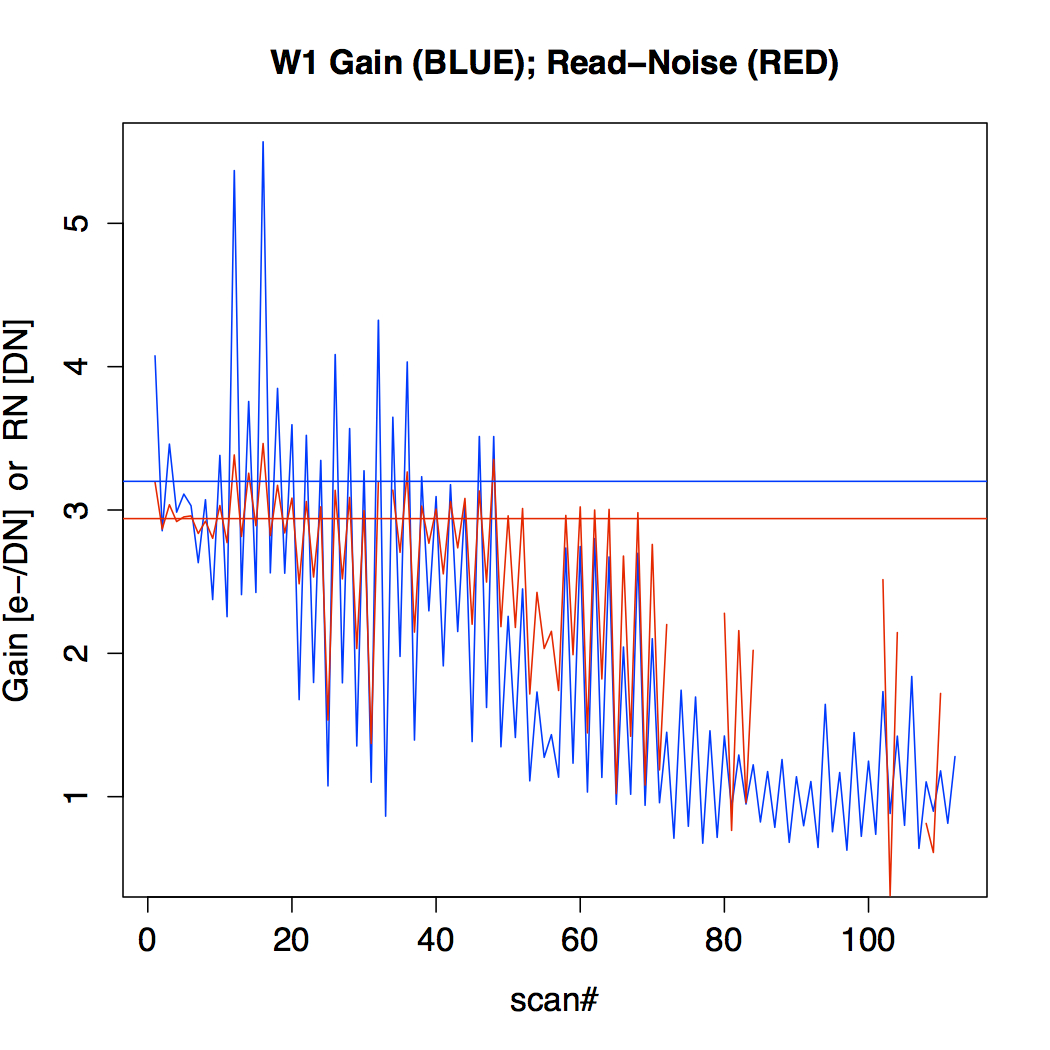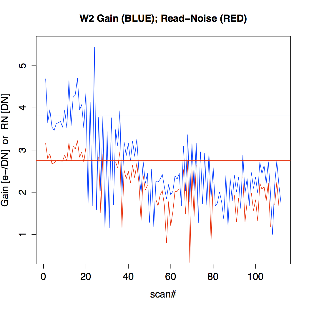Figure 1 - Empirically derived electronic gain and read-noise as a function sequential scan number throughout the 3-band cryo period: W1 (left) and W2 (right). Horizontal lines represent the 4-band cryo "constant" values.

Unlike W1 and W2 where pixel uncertainties were estimated using the error model in section IV.4.a.ii with explicit estimates of the gain and read-noise as a function of time, the W3 pixel uncertainties were dynamically derived. No new gain or read-noise estimates were involved. This is because the W3 detector noise and instrumental signatures changed rapidly throughout the 3-band cryo period as the array temperature increased. Empirical derivations of the gain and read-noise for W3 were not possible. For W3, we resorted to using the gain and read-noise derived from 4-band as priors for the error model, but then the uncertainty pixel map at the end of all instrumental calibration steps was rescaled to match the local RMS in the intensity frame product. This was done robustly by first partitioning the intensity frame into a 10 x 10 grid, and then the partition with the lowest robust RMS was found. This was done to minimize biases from astrophysical structure. The mode of pixel values from same partition in the "errant" uncertainty frame were then computed. The uncertainty image was then rescaled using the ratio: [robust "minimal" intensity RMS]/[mode of unc model prediction]. This scaling was done on a per-W3-frame basis throughout the 3-band cryo period.

The uncertainty frame products were validated against measurements of the RMS fluctuation about the background in the corresponding intensity frames. We used an automated algorithm to select frame background regions that were approximately spatially uniform and had a moderately low source-density. A trimmed lower-tail standard deviation from the mode was used as a proxy for the RMS. This measure was divided by the mode of pixel uncertainties over the same regions to compute a pseudo reduced-χ² measure per pixel. This measure is shown as a function of frame number in Figure 2 for selected scans over the 3-band cryo period and also versus frame pixel median in Figure 3.

Overall, our uncertainty model estimates tracked the noise fluctuations in pixel signals reasonably well over the 3-band cryo period, both in the read-noise limited W1, W2 bands, and the background dominated W3 band. This is consistent with global analyses of PSF-fit photometry to point sources which also show reduced χ² values of ≈ 1 on average for all bands.

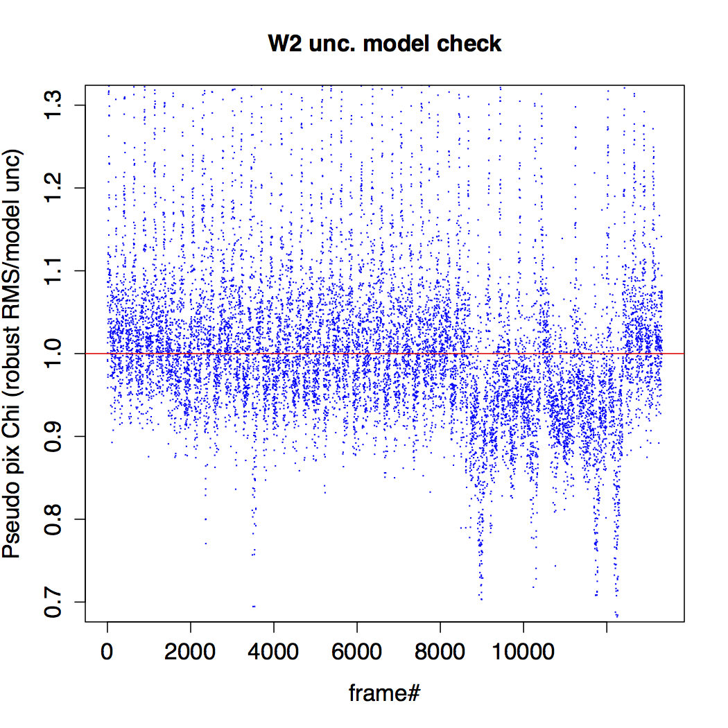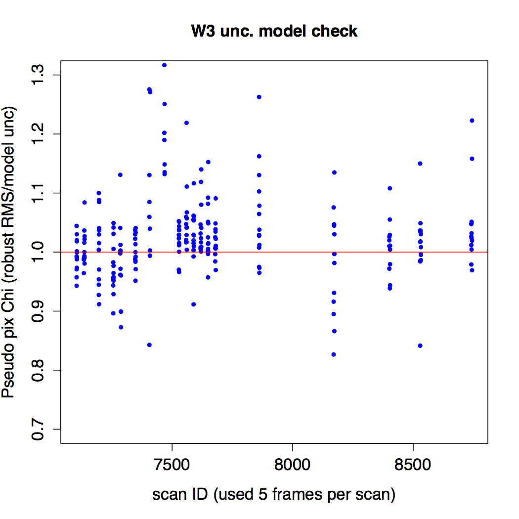Figure 2 - Ratio of "robust pixel RMS/model (modal) pixel uncertainty" versus sequential frame number (from selected scans) over the 3-band cryo period, for W1, W2, W3 (left - right).

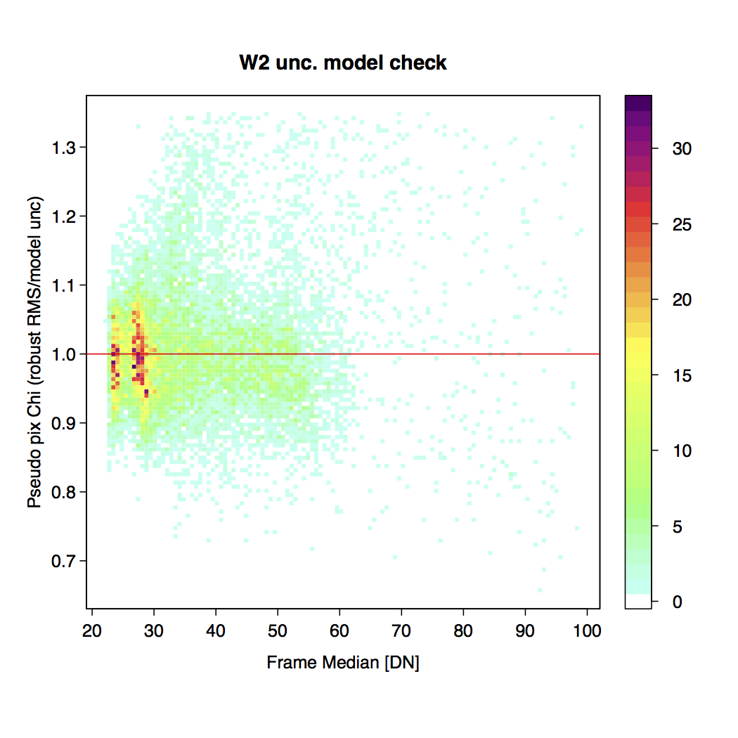Figure 3 - Ratio of "robust pixel RMS/model (modal) pixel uncertainty" versus frame median for ~14,000 frames over the 3-band cryo period, for W1, W2, W3 (left - right).

iv. Bad-pixel Masking and Saturation Tagging

The frame-mask bit-definitions for 3-band cryo were given in section VII.3.b.ii. As in 4-band cryo processing, the frame mask is initialized in the ICal pipeline by first copying all information from the "static" calibration mask into the first 8 bits of a 32-bit buffer (see Table 3) and then setting the dynamic bits as each processing step was applied (e.g., from saturation tagging and dynamic transient pixel tagging within dynacal).

We started with the static calibration masks from 4-band cryo processing and updated them with new bad pixels found from characterizing the 3-band cryo calibrations in each of the 17 intervals listed in Table 2. Most of the new "bad hardware" pixels were found from analysing the time-dependent responsivity maps and their uncertainties inferred from the RMS in image stacks. This allowed us to tag additional pixels with a high or low relative responsivity and/or which were relatively noisy over time. From identifying outlying populations in pixel histograms, the low & high response pixels were tagged using relative responsivity thresholds of <0.7 & >1.5 for both W1, W2, and <0.55 & >1.45 for W3. The RMS uncertainty threshold for declaring a noisy pixel was >2% for W1, W2, and >1% for W3. From the start to the end of the 3-band cryo period, the number of bad pixels flagged according to these criteria increased by factors of ~ 5.7, 2.3, and 2 for W1, W2, and W3 respectively. Figure 4 shows an animation of the evolution in bad pixels flagged over each array in each calibration interval. Corresponding statistics for the number of bad-pixels tagged (and eventually omitted from photometric measurements downstream) are shown in Table 4.

W1	W2	W3
Figure 4 - Click on any panel for an animation of the evolution of the bad-pixel mask over all 3-band cryo calibration intervals. Only "statically set" bad-pixel conditions are shown (static within the calibration interval), i.e., the first 8 bits from Table 3. Statistics are summarized in Table 4.

iv.1. Saturated Pixel Tagging

The saturated-pixel tagging algorithm on board the spacecraft worked reasonably well, however, there were times when it was not reliable and many saturated pixels were not tagged to enable their unambiguous identification during processing. This was most noticeable over the 3-band cryo period where it occurred intermittently when the counts were at the high end of the dynamic range in any band. The values of the mis-tagged saturated pixels were generally much lower than their unsaturated neighbors. If left unmasked, these would have had dire consequences for profile fit photometry (and it did on many occasions, e.g., see cautionary notes in section I.4.b.). 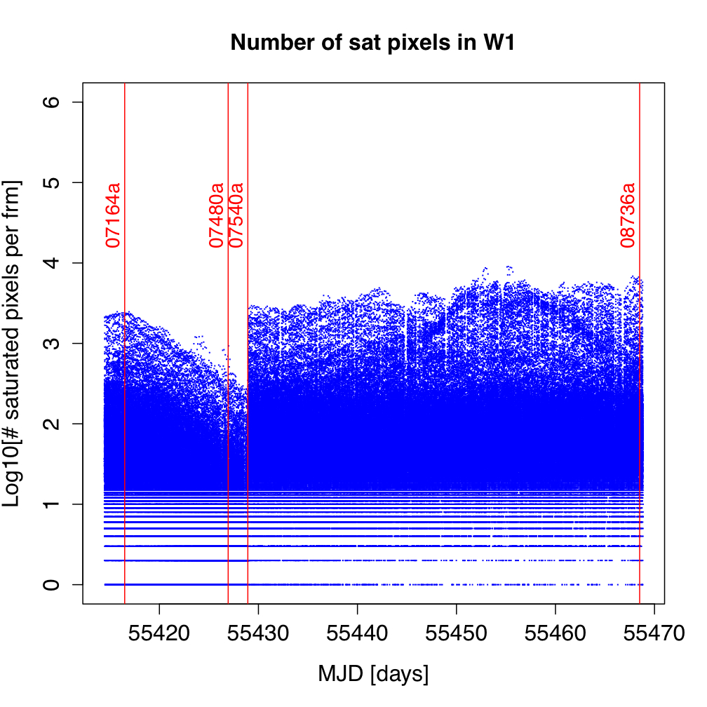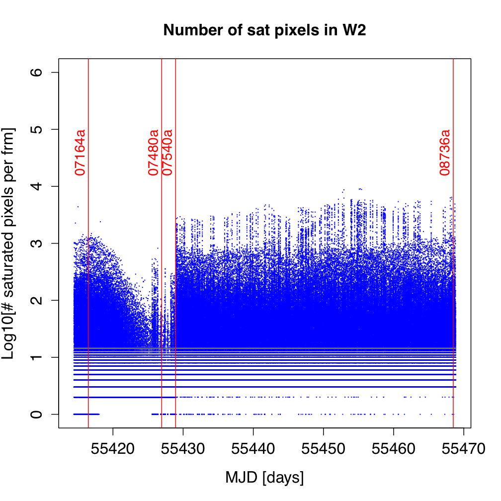For W3, the on-board saturation tagging stopped working with the first exposure-time change (Table 2). Figure 5 shows trends in the saturated pixel count per frame over the 3-band cryo period as reported by the on-board sauration encoding. Note the intermittent losses in the on-board encoding for all bands, in particular for bands W1, W2 where the encoding was operative over a longer span. The intermittent losses in W1, W2 (and total eventual loss in W3) prompted us to develop a brute force saturation masking algorithm. This is described below.

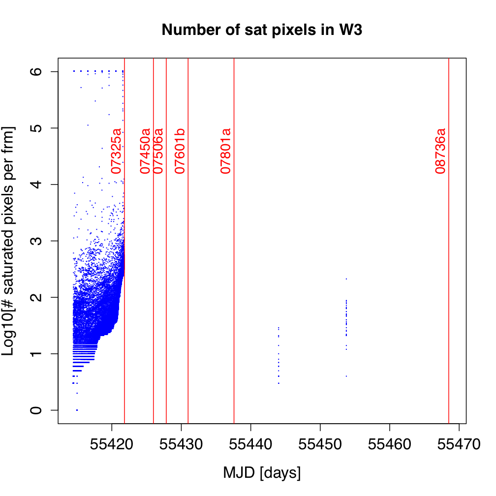Figure 5 - trends in the number of saturated pixels per frame returned by the on-board tagging algorithm for W1, W2, W3 (left - right) over the 3-band cryo period. The vertical red lines with scan IDs mark special events during this period. See the event timeline in section VII.1.a for an explanation.

Forced saturation flagging occurred very early in pipeline processing so all downstream processes would benefit from improved saturation flagging. At this early stage, images had not been calibrated, and no source detection had been performed. Since no purely morphological approach to identifying saturated areas appeared to be feasible, the only available option was to utilize prior knowledge of bright source positions and magnitudes. Fortunately, despite the lack of an extraction list for the images at this stage in the processing, a good source of bright source positions and magnitudes was already on hand: the Bright Source List (BSL) developed for use in artifact flagging. One also needs to have a fairly accurate idea of where a given frame is pointing. Fortunately (again) this information is available from the pass 1 processing.

With these key sources of information at hand, for each frame and band needing it (determined from a reference table), forced saturation flagging proceeded as follows:

• A temporary copy of the level-0 image was created for the band with WCS information updated to reflect the pass 1 position reconstruction.
• The BSL was queried to get a list of positions and magnitudes for all sources within the boundaries of a given frame.
• High proper motion objects from the BSL whose positions were derived from 2MASS had their positions updated to reflect the WISE observation epoch using a preliminary version of UCAC4.
• As was done for artifact flagging, the BSL was supplemented with bright solar system objects within the bounds of the image.
• As for artifact flagging, a best-effort magnitude was determined, drawing from pass 1 measurements, as well as 2MASS and IRAS magnitudes.
• A lookup table (LUT, see below) was consulted to determine the saturation radius for that magnitude.
• Pixels within a circular radius of the size read from the LUT were marked as saturated in the temporary L0 image.

Once saturation was flagged in this way, pipeline processing could proceed as usual, with subsequent steps referring to the modified, temporary L0 image instead of the original. The value 32761 was assigned to pixels in the temporary L0 image to indicate forced saturation flagging. The pipeline then mapped these values to bit #18 in the accompanying mask image (see Table 3).

Forced saturation masking is relatively robust against modest errors in position and magnitude and thus the approximate nature of the BSL information was not generally a hinderance. One class of objects that will likely be under-flagged for saturation are red objects for which pass 1 failed to derive good magnitudes (usually due to, you guessed it, saturation). These objects will have their brightness underestimated in the BSL. Later extraction of these objects will also likely underestimate their magnitudes due to the inadequate saturation flagging. These objects form a tiny fraction of force-flagged objects.

Figure 6 shows the behavior of W3 saturation radius in 3-band cryo estimated by conservatively measuring crater-rim radii in the cores of sources in frames by hand. This is shown as a function of W3 profile-fit magnitude from first-pass processing (i.e., the same processing infrastructure used for the Preliminary Data Release). A good sampling of scans were used from each exposure-time range. The red curve is the prediction from 4-band cryo processing (derived empirically). Aside from the large scatter in Figure 6, this analysis allowed us to calibrate conservative "upper-limit" curves for each exposure-time interval and generate look up tables of saturation radius vs magnitude for tagging saturated pixels during 3-band cryo processing.

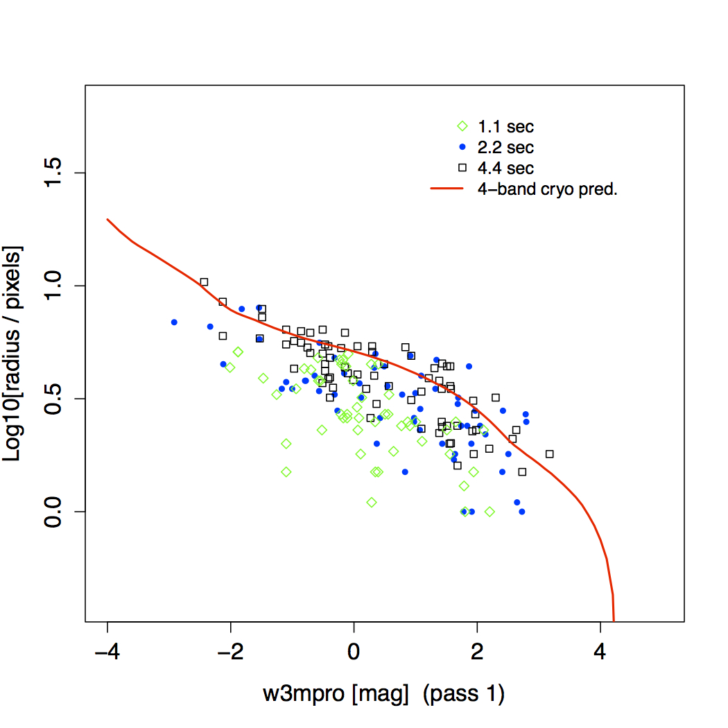Figure 6 - W3 source saturation radius versus profile-fit magnitude from first pass processing.

iv.2. Caveats

It's important to be aware of two limitations with the dynamic saturated pixel tagging:

1. There are many instances of missed saturation. This is mostly seen in regions with bright extended emission.
2. The masking was performed conservatively, that is, more pixels were tagged than needed to be within the cores of sources. This was to ensure the saturated regions were completely tagged and no biases in photometry would result. A consequence of this conservative masking is that as more of the core was masked, more of the wings relative to the core was fit during profile-fit photometry. For reasons not yet understood, fits that placed more weight on the wings appeared to lead to brighter-flux estimates in general. This was also seen for saturated sources in 4-band cryo processing where some flux could be recovered (e.g., Figure 17 in section IV.4.a.vi.1), but to a lesser extent since the nominal saturation tagging used there was not as conservative.

v. Band 3 Droop Correction

The droop correction algorithm is essentially the same as that used in 4-band cryo processing (described in section IV.4.a.iv), but with some enhancements for the "split-droop" correction step. The improvement here is a more accurate pre-calibration of the input frame from which the corrections were derived. This was necessary since the instrumental signatures in W3 were more pronounced in 3-band cryo than earlier in the mission. They were also changing on rapid timescales. In 4-band cryo processing, we prepared the temporary working image by simply subtracting a static dark and dividing by a static responsivity map (see section IV.4.a.iv.1 for details). In 3-band processing, it was necessary to also apply a linearity correction and divide by the dynamically derived flat from dynacal before the split-corrections could be derived. Thresholds for detecting the split-droop effect, in particular in the presence of bright extended structure were also tuned. These changes vastly improved the quality of the droop corrections compared to that achieved in 4-band processing. Examples of before and after droop-corrected frames are shown in Figure 7.

Figure 7 - Collection of 3-band cryo W3 frames where on the top row we show products resulting from processing with the older 4-band cryo droop-correction algorithm, versus those processed with the much improved algorithm applicable to 3-band cryo data (bottom row).

vi. Non-linearity Calibration

We retained the same non-linearity calibration as was derived from ground test data and used to correct the 4-band cryo data. The formalism was described in section IV.4.a.vi with correction formulae (per pixel) given by Equations (18) and (20) therein. The only aspect that changed in 3-band cryo was the value of the coefficient C for W3 (as defined by Eq. 16). This implicitly depends on the Sample-Up-the-Ramp (SUR) weights which were intentionally updated througout the period when resetting the W3 exposure time to avoid saturation after A/D conversion.

For W1 and W2, the adopted linearity calibration was just as accurate as it was for 4-band cryo data, even though the temperature of these arrays increased from the the nominal ~32.2 K to ~ 41.7 K over the 3-band cryo period. Figure 8 compares the photometry (from profile-fitting) of sources from 3-band cryo single-exposures to the same sources measured from 4-band cryo single-exposures. For W1 and W2, there are no signicant differences between these two phases of the mission, across a large range of magnitudes. Due to the paucity of sources in W3, especially at the shortest exposures, the comparison to 4-band photometry in Figure 8 is not very informative. However, it illustrates the degree at which the flux limit (at fixed S/N) became brighter as the W3 exposure-time was shortened. These limits were derived empirically from the calibrated data and accounted for all instrumental variations throughout the 3-band cryo period. See below for a more in-depth characterization of W3.

W1	W2	W3
Figure 8 - Single frame 3-band cryo (v4) - 4-band (v4.5) photometry from profile-fitting as a function of 4-band photometry for W1, W2, W3 (left - right). The W3 results are broken down by exposure time and approximate magnitude limits corresponding to S/N ~ 5 are also shown.

It was very difficult to validate the accuracy of the non-linearity calibration for W3 within the time-frame available prior to 3-band cryo processing. Little did we know that the large temperature variations would have a significant impact on the W3 linearity, in particular as a function of position on the array (see below). For this band, significant spatial residuals remain in the single-exposure frames. This has adversely affected the single-exposure photometry, mostly in a relative sense, i.e., when the same source is measured at different locations on a frame. These biases are partially washed out in multiframe profile-fit photometry when stacking a relatively large number of frames (e.g., with depth-of-coverage >~ 20), although the variance across a stack (at a fixed sky position) is appreciably inflated compared to 4-band cryo measurements. This makes the 3-band cryo W3 single-exposure photometry unsuitable for variability studies. For example, if one plans to use relative photometry to search for astrophysical variations of amplitude <~0.2 mag in W3 sources at >4.0 mag (conservatively speaking). See below for details.

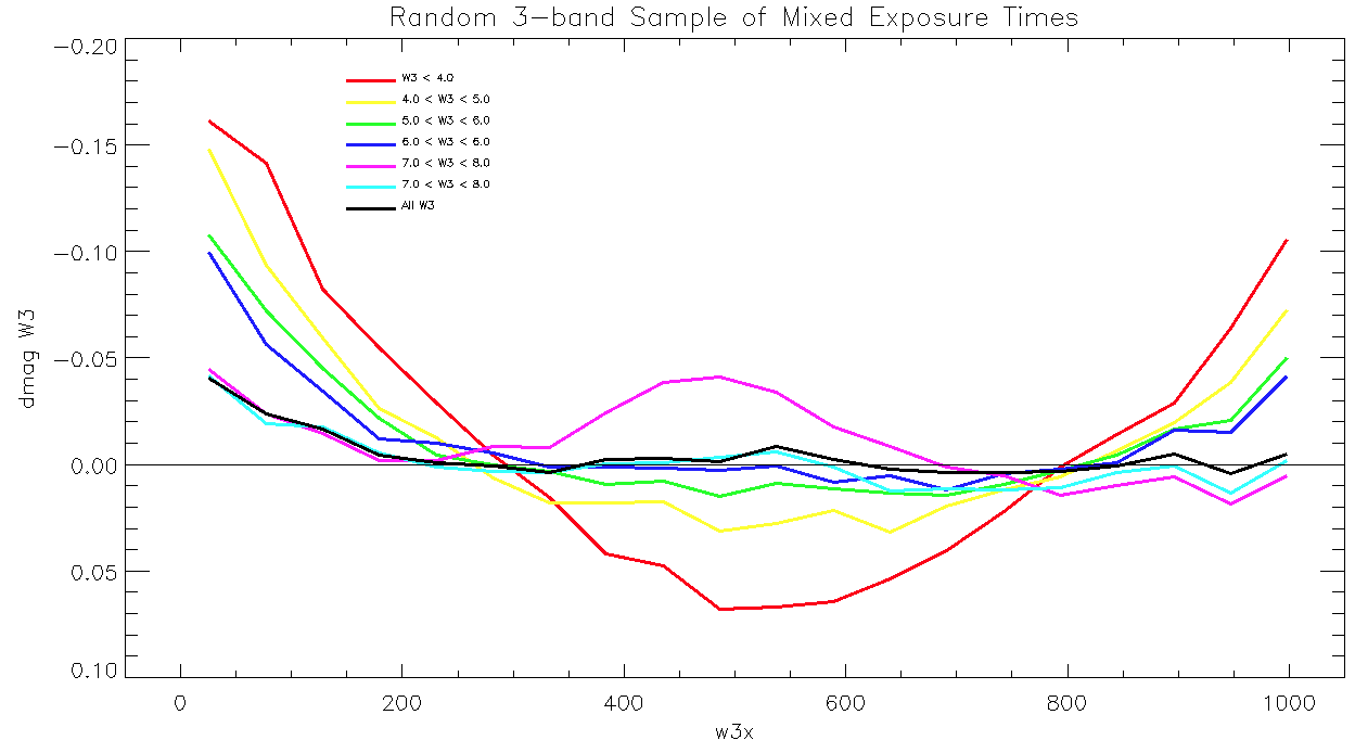
The linearity-calibration residuals were characterized by exploring the light-curves of single W3 sources as a function of their x pixel position in the frame. Similar results are obtained as a function of y. The majority of W3 light curves during the 3-band cryo period are brightest near the beginning and end of their observation window (i.e., spanning all the multiple single-exposure apparitions). This directly correlates with the location of the source on the focal plane as the source passes from edge to edge over the observation window. Analyses have shown that the residuals increase as the source flux increases, consistent with an "over-correction" for linearity since in general, the magnitude of this correction is always relatively larger for brighter signals. The residuals also increased as the exposure time was decreased during the 3-band cryo warm-up. The effect is not seen in 4-band cryo, nor in W1 and W2.

Figures 9a - 9b demonstrate the above mentioned effects. These figures were generated by first querying 100,000 sources from the 3-band multi-frame source catalog that had (w3mjdmax - w3mjdmin) < 5.0 and cc_flags = '0000'. The latter was to minimize contamination by artifacts. The time-span constraint ensured the sources were only observed during one epoch and not contaminated by moon-toggles. For the 8.8 sec-only and 1.1 sec-only exposure-time plots (Figures 8c and 8d), the source also had to be observed solely within the appropriate exposure-time period. Next, the list of 100,000 objects were cross-matched to the single-exposure source data via a 2.5 arcsec cone search. For each coadd-detected source, the mean of the corresponding single-exposure W3 flux measurements was then subtracted from each individual flux measurement, therefore normalizing the light curve. The resulting residuals are referred to as dmag in Figure 9. The sources were then binned by x-position on the array, and also by mean W3 magnitude. The median dmag value within each bin was then plotted.

Figure 9a - Median deviation from the mean flux level as a function of x-position on the detector and mean magnitude for a random sample of 100,000 W3 sources throughout the 3-band cryo period.	Figure 9b - Median deviation from the mean flux level as a function of x-position on the detector and mean magnitude for a random sample of 100,000 W3 sources during the nominal 4-band cryo period.
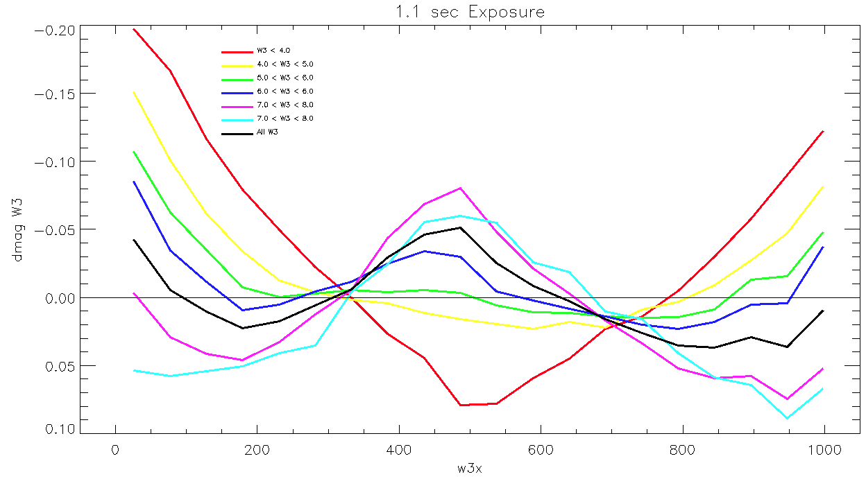Figure 9c - Median deviation from the mean flux level as a function of x-position on the detector and mean magnitude for a random sample of 100,000 W3 sources picked exclusively from the period with 8.8 sec exposures during 3-band cryo.	Figure 9d - The same as Figure 8c, but limited to the 1.1 sec exposure-time period during 3-band cryo.

vii. Relative Responsivity (Flat-field) Calibration

As for the 4-band cryo calibrations (section IV.4.a.vii), flat-fields for the 3-band cryo period for W1, W2, and W3 were created directly from the survey data. Due to the continually changing telescope and focal plane temperatures during this period, separate calibrations were derived for each of the 17 intervals defined in Table 2. The selection of these intervals were driven by various factors, such as W3 exposure-time changes to avoid severe saturation, and the availability of sufficient post-anneal data for W3 in a given period.

Flat-fields for each time interval were created following the same methods as described in section IV.4.a.vii. The resulting flat-field images for each interval are shown in Figures 10, 11, and 12 for W1, W2, and W3 respectively. Changes in the spatial structure of the responsivity with time are evident. In addition, some W3 flats contain obvious long-term latent residuals due to the limited amount of data that could be used within the intervals. These "static" residuals were mitigated by applying dynamic "delta-flat" corrections per W3 frame as described in section VII.3.b.viii.

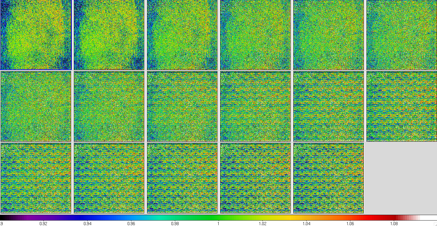Figure 10 - W1 relative responsivity maps for the 17 3-band cryo intervals defined in Table 2. Time increases from the top-left to the bottom-right image.

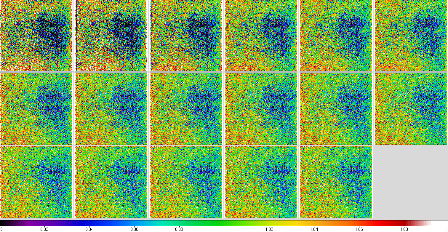Figure 11 - W2 relative responsivity maps for the 17 3-band cryo intervals defined in Table 2. Time increases from the top-left to the bottom-right image.

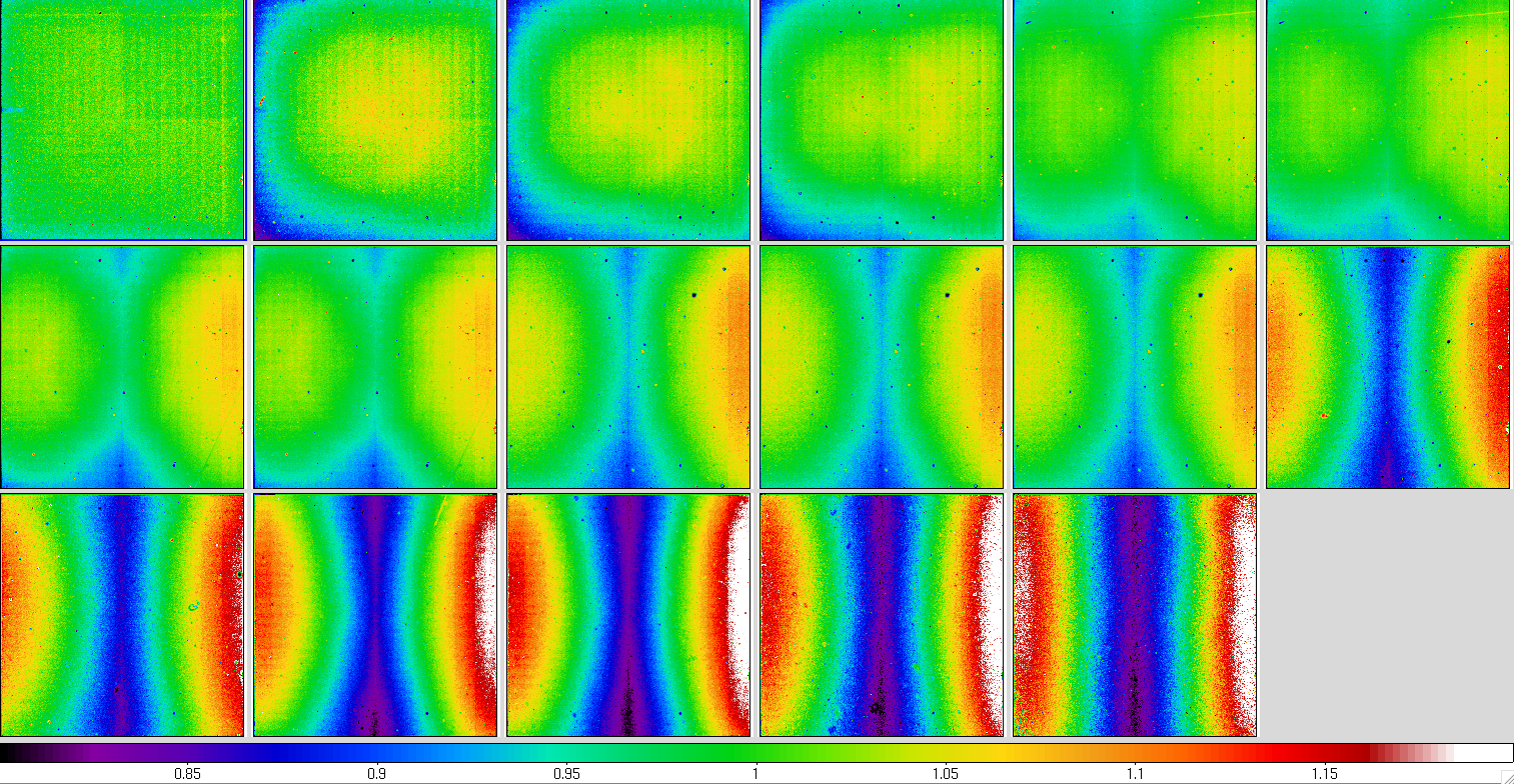Figure 12 - W3 relative responsivity maps for the 17 3-band cryo intervals defined in Table 2. Time increases from the top-left to the bottom-right image.

An estimate of the flat-field accuracy is provided by the relative percent uncertainty derived from the accompanying uncertainty images. This is defined as the median of 100*[σ(f) /f] over all the pixels where σ(f) is the 1-sigma uncertainty in the responsivity f for a pixel. The median relative percent uncertainties for all calibration intervals are listed in Table 5.

viii. Dynamic Calibration

The purpose of dynamic calibration (dynacal) is to capture instrumental transients in the detectors and then correct them in the frames from which the dynamic calibrations were made, or at least in frames not too far in time from the time-dependent calibration. 3-band cryo processing used the same dynacal methodology as in 4-band cryo, as outlined in section IV.4.a.viii.

The dynacal products generated in 3-band cryo were: (i) sky-offsets for W1, W2, and W3; (ii) delta flat-field (or residual relative pixel resposivity) corrections for W3 only; and (iii) detection and tagging of bad-pixel transients in the frame masks for W1, W2, and W3. The only difference from 4-band cryo processing is that full-frame pixel responsitivity maps were computed dynamically for W3 throughout the 3-band cryo period, instead of just thresholded low-frequency versions as in 4-band cryo. The goal of the latter was primarily to correct spatially extended enhancements in responsivity brought about by long-term latents. In 3-band cryo, the intent was to also catch general variations in the relative responsivity on timescales faster than those defined by the fixed calibration intervals in Table 2.

The dynamic sky-offsets and delta-flats were computed by combining pre-calibrated frames that were dark subtracted, linearized, and flattened using the "static" calibrations from each interval in Table 2. The pre-processing steps (some of which are band-dependent) are outlined in Figure 1 of section IV.4.a.i. The dynacal products were then made be collapsing the pre-calibrated frames using single frame-step moving medians within windows of length 37 for W1 and W2, and 43 for W3, with minimum lengths of 29 for W1 and W2, and 35 for W3 to allow for filtering of bad frames. Below these minima, dynacal assigned the best calibration product that was closest in time to the frame in question. The frame-filtering thresholds for noise, illumination level and cosmic-ray count for omitting frames from the dynacal windows were also specially tuned for 3-band cryo processing.

viii.1. Caveats

Overall, the dynamic calibrations kept the frame processing sane, catching occasional transients and changes in instrumental signatures reasonably well, particularly in W3. Two caveats were discovered when examining the frame products: first, the W3 dynamic calibrations did not work well for ~15 - 20 frames on either side of each "static" calibration interval defined in Table 2. The discontinuous nature of the pre-calibrations across these boundaries resulted in inaccurate dynacal products. This occured 16 times (for the 17 "static" calibration intervals) and resulted in ~350 frames containing significant latent and flat-fielding residuals across the 3-band cryo period. Given the affected W3 frames fell at the start and end of scans, they will have occured when observing near an ecliptic pole where suppression in multiframe processing would have beeen maximal.

The second caveat results from a consequence of including the actual frame on which a dynacal product was applied in the dynacal frame-stack itself. This resulted in an excess of pixel values around the stack median in the final processed frame. This excess is discerned as a spike in the pixel histogram. Given a finite number of N_w frames in a window are stacked, a fraction 1/N_w of the pixels in the frame will inevitably equal the median exactly by chance. This is because the median will pick-out discrete values equal to one of the input measurements when the number of inputs is an odd integer. This anomaly occured throughout the mission (both 3-band and 4-band cryo phases) and has lead to biases in the photometery as described in section VI.3.c.. The impact was mostly to W1 and W2 photometry, while the higher backgrounds in W3 had a tendency to suppress the effect.

In general, all the cautionary notes listed in section I.4.d.6 apply here, except the last bullet point related to dynacal. Given the W3 delta-flats in 3-band cryo are full-frame pixel responsivity maps (as opposed to low-frequency thresholded versions in 4-band cryo), edge residuals are not seen in the 3-band cryo frame products.

Last update: 2012 July 27