IV. WISE Data Processing

4. Pipeline Science Modules

g. Artifact Identification and Flagging (ARTID)

Contents

Bright stars produce a number of artifacts in the both the single exposure and atlas images. These artifacts include diffraction spikes, scattered-light halos, optical ghosts, persistence (latents), and glints. What follows is a description of each artifact, the characterization and flagging procedure in single frame (scan frame) and multiframe (atlas) images, and procedure for refinement of parameters. In single-frame images (i.e., scan frame or Level 1b images), diffraction spikes (flag='d'), halos (flag='h'), ghosts(flag='o'), latents (flag='p'), and glints (flag='g') are flagged. Upper-case flags in the 'cc_flags' field represent spurious sources, which exist solely due to the artifact, and lower-case flags represent real astrophysical objects whose photometry is contaminated by the artifact. The only exception to this convention applies to the flagging of glints, In multiframe flagging (i.e., atlas images) all artifacts except glints are flagged (see below for an explanation). We strongly recommend that you familiarize yourself with the cautionary notes in this section before using the cc_flags field in your searches.

The version of ArtID used for the All-Sky Data Release incorporates numerous improvements over previous versions (including the version used for the Preliminary Data Release). One of the major additions is the flagging of artifacts created by parents which lie off-frame. I.e., when a bright parent falls just outside of the single-frame or atlas image, its diffraction spikes, halo, ghosts, etc. may still extend into the frame in question. This is, in fact, always true of "glints" in single-frame images, which are caused when a bright parent lies just outside the frame. In order to facilitate the flagging of artifacts with off-frame parents, ArtID makes use of a bright source list, which includes stars which are bright enough to create artifacts. For each frame, ArtID searches the bright source list for sources in the surrounding area which may produce artifacts in the frame, and flags them as necessary. The bright source list is also used to supplement the list of latents parents and to supplement the WISE photometry for more accurate flagging when the extracted WISE photometry was underestimating the flux of extremely saturated stars.

Other changes include the addition of background-dependent spike and halo sizes and adjustments for high ecliptic latitude effects on the artifacts.

i. Diffraction Spikes

Diffraction spikes are linear features caused by diffracted light from the telescope's secondary mirror support structure. In a single frame image, they extend from a bright source at angles of approximately 45, 135, 225, and 315 degrees, where 0 degrees is aligned with the positive y-axis (see Figure 1). Diffractions spikes also appear in atlas (coadded) images, though they are somewhat mitigated at high ecliptic latitudes where their positions angles on the sky vary due to the nature of the spacecraft's orbit. Flagging of sources created or contaminated by diffractions spikes is similar in the single-frame and atlas images; however, there are important differences outlined in the section below.

i.1 Single-frame Flagging

i.1.a Spike Lengths and Widths

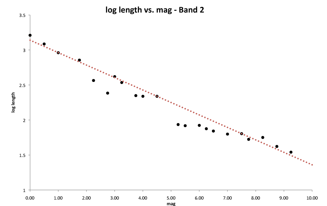
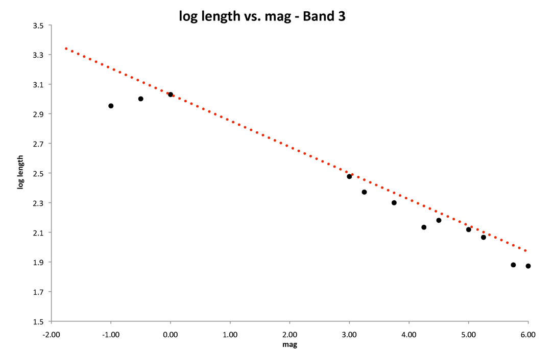
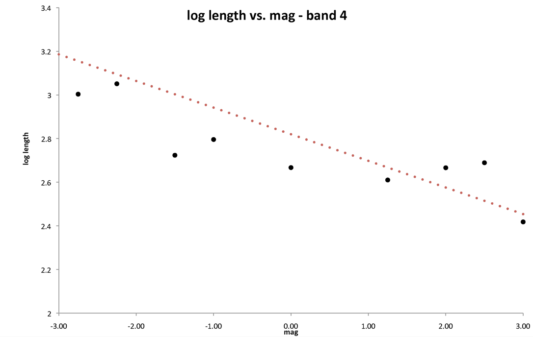
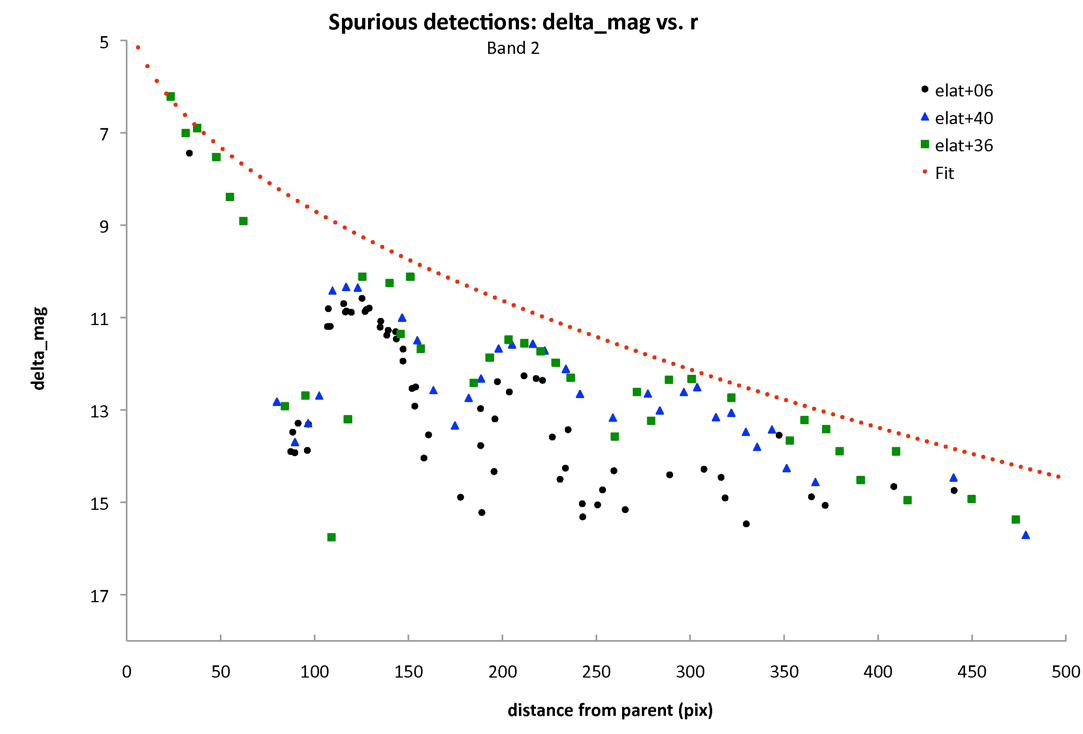
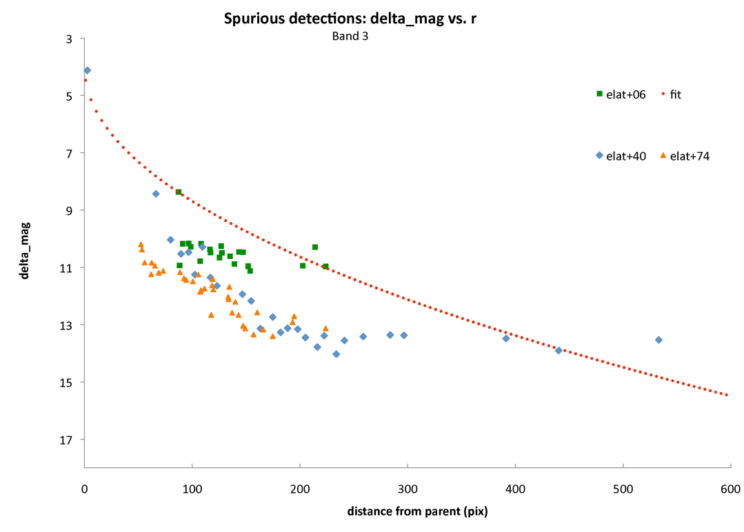
The size (length and width) of a diffraction spike is determined by the brightness of the star producing the spike (referred to as the "parent" star). In order to flag sources which are created by diffractions spikes ("spurious" sources), as well as astrophysical sources that have their photometry contaminated by diffraction spikes, we employ empirically-derived functional relations to predict spike length and width as a function of parent star brightness (Figure 1). In order to derive a functional form relating the spike length, L_S, and spike width, W_S, to parent magnitude, m_p, a series of "source-space" images, generated using source extractions from WISE images. This is accomplished in the following manner: For a bright source that produces diffraction spikes, the positions of the surrounding source extractions are plotted. This produces a source-space image for one parent. This process is repeated for a large number of parents in a given magnitude bin, and the resulting source-space images are then stacked (typically thousands of stars per magnitude bin, but significantly fewer, down to a few, for the brightest objects), with a common center for the parent stars. This produces an composite source-space image for a given magnitude bin (Figure 2). The length of the diffractions spikes are determined by inspection of the composite source-space image for a range of parent magnitude bins. Figures 3 through 6 show the diffraction spike length vs. parent magnitude plots for each of the four bands, as well as the fits used for flagging. The functional form of the equation relating L_S to m_p is:

where L_S is in arcseconds. The values of the parameters 'a_L' and ' b_L' are shown in Table 1. Table 1 also lists the threshold values for parent brightness (in mag) for diffractions spikes in each band (i.e., the brightnesses for parents at which diffraction spikes begin to appear).

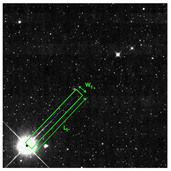Figure 1 - Example of a diffraction spike. Also shown are the size parameters used to flag sources.

Note that in all cases, the fit tends to lie above the data points. This is because the best fit was chosen to err on the side of overflagging; that is, the functions estimate the spike lengths to be somewhat longer than the actual spikes. The purpose of this is to ensure that real sources lying at the faint ends of the spikes are flagged as potentially contaminated. Since our initial evaluation of spike lengths were done using source-space images, the derived values are dependent on spurious sources being extracted from the diffraction spikes. At the faint end of the diffraction spikes, it is possible that no spurious extractions are being made, but there may still be a low level of flux capable of contaminating the photometry of real sources. Some minor overflagging is likely to occur because our parameters are tuned in this way, but this was done to ensure all affected sources were flagged. Another note that the source-space images used in the determination of spike lengths were generated using coadded images prior to the WISE Preliminary Data Release (the fits are nearly identical as well). As it turns out, these fits do a fairly good job of reproducing the diffraction spike lengths for the single-frame and atlas images in the All-sky Data Release, when combined with the newly incorporated background-dependent scaling described below.

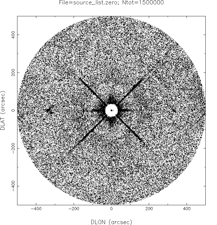Figure 2 - Example of a source-space image used to evaluate spike lengths and widths. This particular image is for the magnitude 3.75-4.00 bin in Band 1, and is about 1000 arcseconds on a side.

Figure 3 - Plot of spike length (LS) vs. mp for Band 1. The black data points have been determined from the source-space images, as described in the text. The red dotted line indicates the fit, which is chosen to lie above most of the data points.	Figure 4 - Same as Figure 3, but for Band 2.
Figure 5 - Same as Figure 3, but for Band 3.	Figure 6 - Same as Figure 3, but for Band 4.

We also evaluate the parent star brightness at which spikes no longer appear, m_{thr_d}, for each band. This is also done using the source space images. Spikes are considered to have disappeared once their lengths are well inside the radius of the halo. We list the final values of a_L, b_L, and m_{thr_d} below in Table 1.

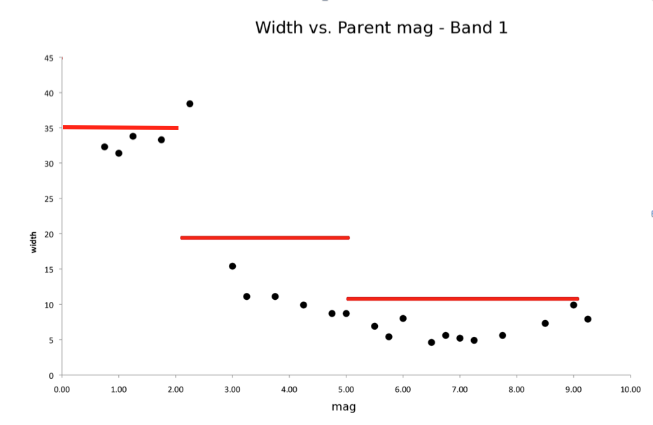
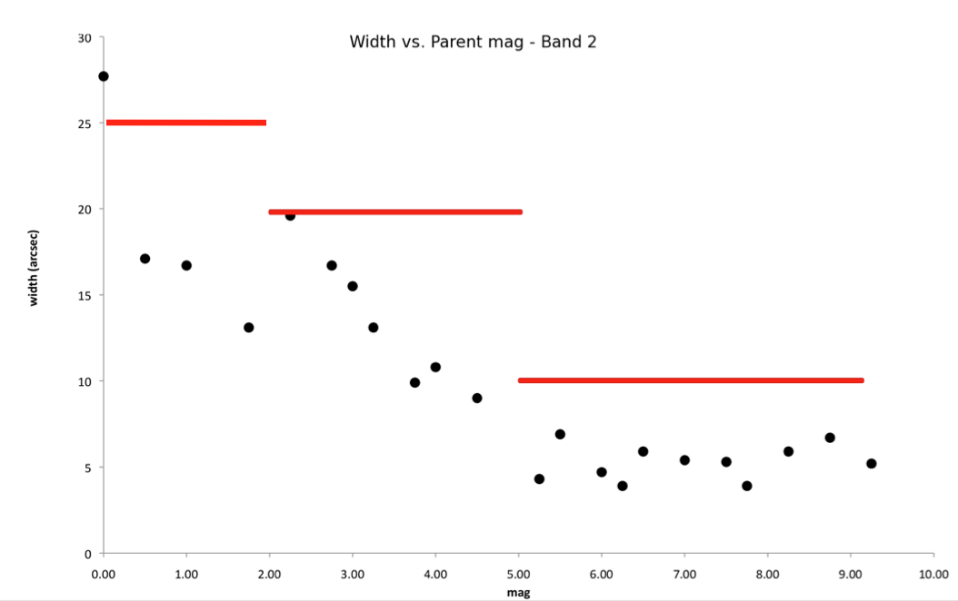
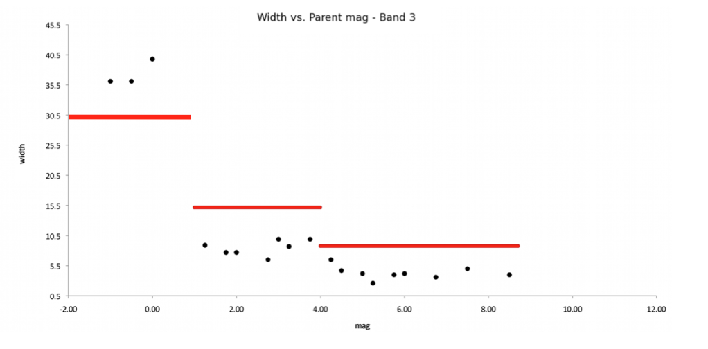
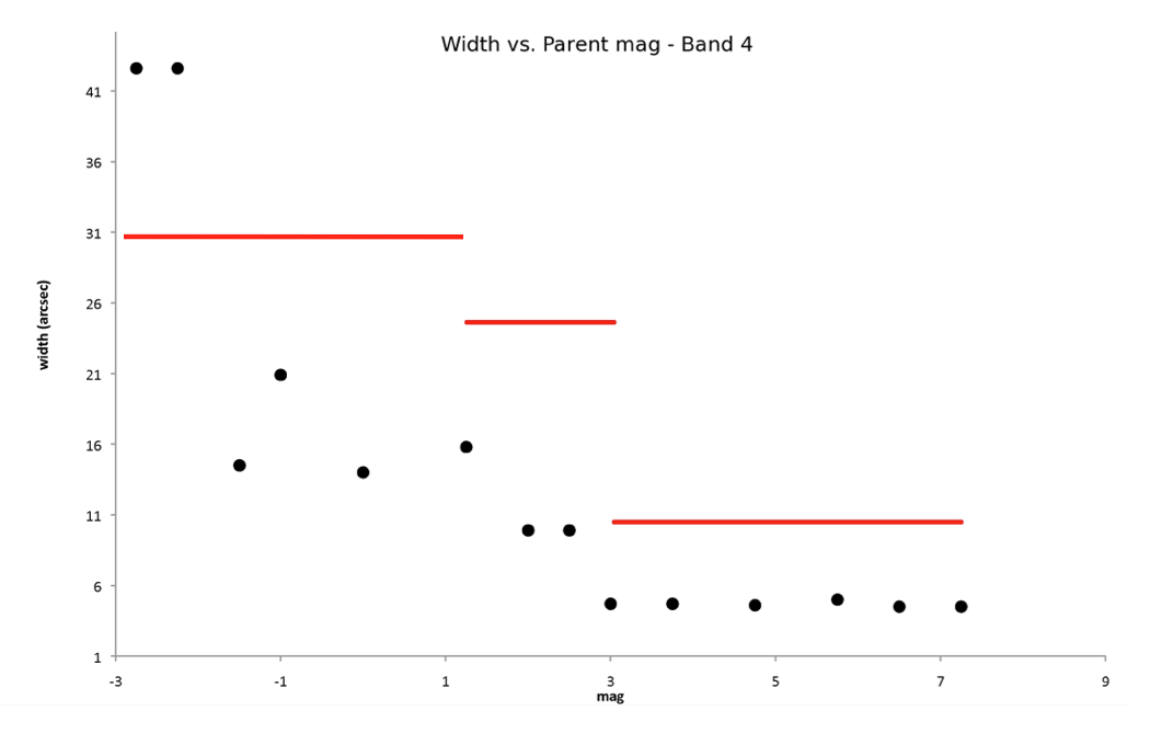
Spike widths are determined in a similar manner to spike lengths. Given the relative lack of dependence W_S shows over small changes in parent magnitude, the functional form used is a step function. Figures 7 through 10 show the W_S vs. m_p relations for each band. The parameters used in flagging are shown in Table 2. In general, the brightest parents were ignored when determining the values of the parameters, as these objects were very rare, and using such large values for spike width lead to significant overflagging for the vast majority of sources.

Figure 7 - Plot of spike width (WS) vs. mp for Band 1. The black data points have been determined from the source-space images. The red lines indicate the step functions used in the flagging. Widths are given in arcseconds.	Figure 8 - The same as Figure 7 except for Band 2.
Figure 9 - The same as Figure 7 except for Band 3.	Figure 10 - The same as Figure 7 except for Band 4.

i.1.b Spurious sources vs. Real/Contaminated sources

Two types of sources are flagged by ArtID, those that exist purely as a result of an artifact, referred to as spurious sources (and flagged with a capital letter, in the case of diffraction spikes, 'D'), and those that are real astrophysical objects, but whose photometry are contaminated by flux from an artifact (flagged with a lower-case letter, 'd' in the case of diffraction spikes). For the purpose of determining whether a flagged source is spurious or real, we assume that a given artifact can produce spurious extractions up to a given brightness, dependent primarily upon the brightness of the parent star, m_p. The brightness of the brightest spurious extraction can be generally given by an expression m_p + Δm_{spur_d}, where Δm_{spur_d} is the magnitude difference between the brightest spurious source and the parent. Whether a flagged source is flagged as spurious or contaminated is determined by whether the source in question is brighter or fainter than this threshold. If a flagged source with magnitude m_s is fainter than the threshold value (m_s &ge m_p + Δm_{spur_d}) then the source is assumed to be spurious. If a flagged source is brighter than the threshold value (m_s < m_p + Δm_{spur_d}) then the source is flagged as real and contaminated.

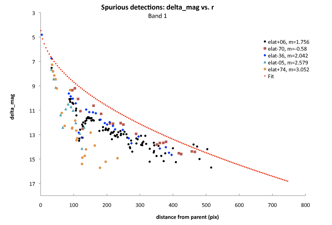
The functional form describing the behavior of Δm_{spur_d} for diffraction spikes was initially determined for flagging of atlas images in the WISE Preliminary Data Release. For this initial determination, we utilized a set of 15 test coadds, from which we selected about 30 bright sources in all bands. We assumed that the value of Δm_{spur_d} depended on the distance from the parent star. For each of the bright parents, the magnitudes of spurious extractions along the spike were plotted as a function of distance from the center of the parent. Our analysis used over 500 spurious extractions in all bands. The nature of the spurious extraction was verified by eye to ensure that no real sources were included. The Δm_{spur_d} vs. r_parent plots are shown in Figures 11 through 14. Table 3 shows the adopted values for the All-Sky release single-frame flagging.

The function relating Δm_{spur_d} to r_parent was determined, following the general form:

where a_spur, b_spur, and c_spur are the parameters to be determined.

The functional forms remain the same for the All-Sky Release single-frame flagging, though the parameters have been adjusted based upon inspection of single-frame test runs. In general, the value of Δm_{spur_d} is set artificially high, to ensure that all spurious sources are flagged as such, to favor catalog reliability. The negative impact is that real sources lying along the spikes may be flagged as spurious, and not included in the All-Sky Catalog.

Figure 11 - A plot of Δmspur_d for spurious extractions along the spikes of several bright parent stars (each symbol representing a different star), spanning a range of ecliptic latitudes in Band 1. A functional fit is also shown (red dotted line).	Figure 12 - The same as Figure 13 except for Band 2.
Figure 13 - The same as Figure 13 except for Band 3.	Figure 14 - The same as Figure 13 except for Band 4.

i.1.c Background Level Dependence

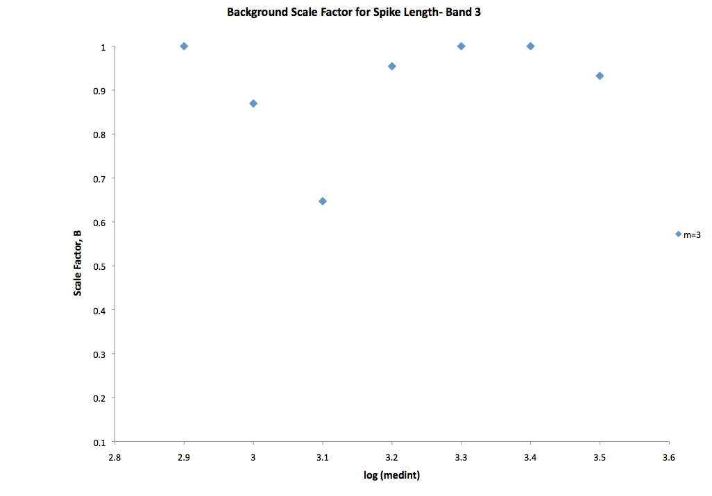
A major addition to the flagging of diffraction spikes in the All-Sky Release is the incorporation of background level dependence in the determination of spike lengths. It became clear in the flagging of diffraction spikes for the Preliminary Data Release, that the model used to predict spike lengths was over-simplified. One of the components missing from the Preliminary Release model was the dependence of diffraction spike length on the background level of the frame where the spike appeared. In frames with a high background level, spikes tend to be shorter, as the faint ends of the spike drop below the level of noise at a smaller distance from the parent star. Thus, where background levels are high (in the galactic plane, for example), the lengths of spikes are significantly overestimated by the model, leading to gross overflagging in frames with high background levels.

In order to mitigate this effect, we incorporate background dependent scaling for diffraction spike lengths. For frames with high background levels, diffraction spike lengths are reduced by a multiplicative scale factor. In other words, the background corrected diffraction spike length, L_{S_bg}, is related to the original spike length, L_S by the relation:

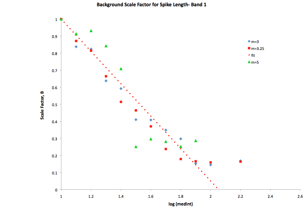
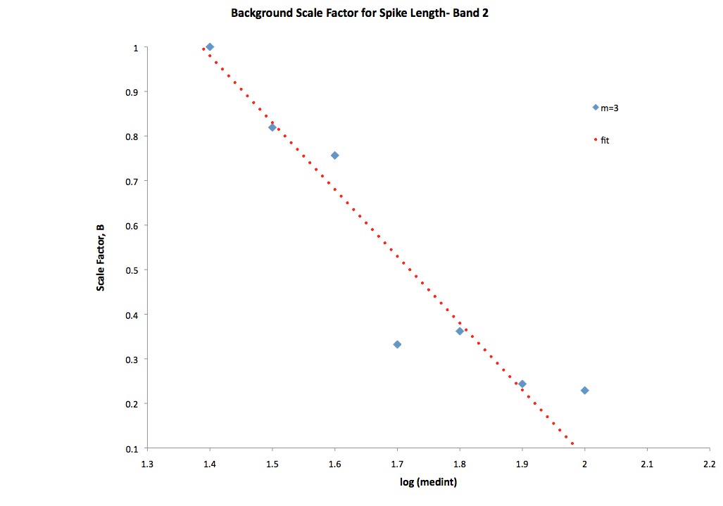
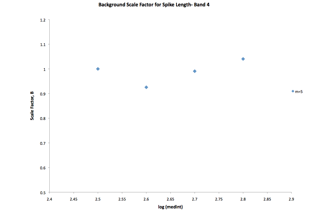
Where 'B' is the background scaling factor, generally a value between 0 and 1. The dependence of 'B' on background level is determined empirically. For each band, we generated a series of composite source space images, in a manner similar to the procedure described above for determining the parent magnitude dependence of the spike lengths. In this case, however, we binned the parents by background level of the frame (the frame's value of 'medint' is used as a proxy for background level), in addition to their magnitude. The lengths of the diffraction spikes in each medint and magnitude bin by inspection of the source space image. Figures 15-18 show the results of this analysis for each band. Values of log(medint) are plotted along the x-axis, while the ratio of actual spike length (determined using the source-space images) to predicted spike length (from the non-background-corrected model) are plotted along the y-axis, the latter being essentially the empirically determined value of B. The relation between B and log(medint) is well-fit by a line:

where 'c_bg' and 'd_bg' are the parameters to be determined. For single-frame flagging, we determined that only Bands 1 and 2 displayed a significant variation for spike length with respect to background level. Thus, the parameters for Bands 3 and 4 were set so that no background-dependent scaling was applied to the final spike length. We also set minimum and maximum possible values for B.

Figure 15 - B vs. log(medint) for Band 1. Parents of different brightnesses are represented by the different symbols. The red dotted line shows the fit.	Figure 16 - B vs. log(medint) for Band 2. The red dotted line shows the fit.
Figure 17 - B vs. log(medint) for Band 3. No significant trend is apparent.	Figure 17 - B vs. log(medint) for Band 4. No significant trend is apparent.

i.1.d Secondary Spikes (Band 3)

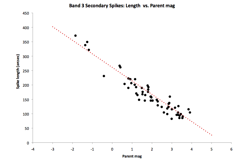
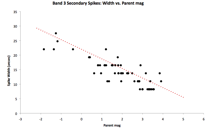
Aside from the diffraction spikes at 45, 135, 225, and 315 degrees, bright sources in Band 3 often show prominent spikes at the 0, 90, 180, and 270 degree positions (referred to as "secondary" diffraction spikes). For the WISE All-Sky Data Release, these spikes are flagged in Band 3 only. Characterization of the lengths and widths of these spikes was performed independently of the primary diffractions spikes. As with the primary spikes, we determine functions which relate the spike length and width (L_sec and W_sec) to parent magnitude. Plots of L_sec vs. m_p and W_sec vs. m_p were created for 58 bright Band 3 sources ranging in brightness from -2 to 4 mag. The objects were also chosen from single-frames spanning a range of background levels. Unlike primary spikes, the background level of the frames was not found to have a significant effect on the spike size. This is possibly due to the relatively short lengths for these spikes. The lengths and widths were determined to be well fit by simple linear relations:

The values of parameters resulting in the best fit, erring slightly on the side of overflagging, are given in Table 5, and the plots for length and width are shown in Figures 19 and 20.

Figure 19 - A plot of Lsec vs. mp for 58 objects in Band 3, spanning a range of parent magnitude and background levels.	Figure 20 - A plot of Wsec vs. mp for 58 objects in Band 3, spanning a range of parent magnitude and background levels.

i.2 Multiframe Flagging

Flagging of diffraction spikes in the multiframe pipeline (which generates the final atlas images) is very similar in nature to flagging in the single-frame images. Flagging of diffraction spikes in the multiframe pipeline is based on the same initial characterization of spikes performed for the single-frame flagging. Please see the appropriate section in the single-frame section above for a description of the initial characterization. The initial characterization provided values for the parameters which were used as a starting point in the multiframe version of ArtID (i.e., the single-frame parameters were initially used for the multiframe flagging). Test runs of the multiframe pipeline produced several hundred test images which were inspected, and adjustments to the diffraction spike length and width parameters were made. Several iterations of inspection and refinement of the parameters were performed.

The major additions in multiframe flagging of diffraction spikes are: 1) The use of depth-of-coverage scaled magnitudes for parents stars and 2) the addition of high ecliptic latitude diffraction spike length scaling. These additions are described below.

i.2.a Depth-of-coverage Scaling of Parent Magnitudes

When images are coadded together, the signal-to-noise of detected sources is increased by a factor of n^1/2 compared to the single-frame images, where 'n' is the number of frames which are coadded together. This is true of both real astrophysical objects as well as artifacts, when they lie at the same "on-sky" position in each of the single frames. In general, diffraction spikes coadd in this manner (with the exception of spikes at very high ecliptic latitudes; see section below on high ecliptic latitude scaling). Thus we expect diffraction spikes to be longer in the coadded images compared to the single-frames. We attempt to account for this effect by assuming a parent star is brighter by a factor of n^1/2 than its actual magnitude. For the value of 'n' we use the 'w?cov' value which describes the number of single-frame coveages for the appropriate band at the location of the parent. This adjustment is not ideal, but to first order does a good job of adjusting diffraction spike lengths to account for depth-of-coverage. All parameters in the multiframe version of ArtID are refined to optimize performance of flagging with the scaled magnitudes.

i.2.b Lengths, Widths and Spurious vs. Real Determination

Length and width parameters were refined for multiframe flagging, as described above, and remain largely unchanged. For a description of the initial characterization and functional forms of diffraction spike length, width, and spurious/real determination, we refer the user to the section that describes the single-frame flagging of diffraction spikes. Tables 6 and 7 list the length and width parameters, while Table 8 lists the parameters used for spurious/real determination.

i.2.c Background Dependence

Background-dependent scaling parameters were refined for multiframe flagging, as described above. In the coadded images, diffraction spikes in Bands 3 and 4 show a weak dependence for spike length vs. background level (the single-frame images did not show such a variation). As a result, background-dependent scaling for these bands are now included. For a description of the initial characterization and functional forms of the background-dependent scale factor, we refer the user to the section that describes the single-frame background-dependent scale factor for flagging of diffraction spikes. Table 9 shows the parameters used in multiframe flagging.

i.2.d Spike "Fanning" and High Ecliptic Latitude Length Scaling

At high ecliptic latitudes, diffraction spikes behave differently in a coadded image (such as the Atlas images). Due to the nature of the WISE orbit, regions near the ecliptic poles have high coverage (i.e., many single images are taken of the same piece of sky), and these single images span a range in position angle for any given piece of sky (i.e., the telescope is rotated differently with respect to the sky). Since the orientation of diffraction spikes are tied to the secondary support structure, and hence fixed with respect to the detector, the orientation of the diffraction spikes with respect to the sky will also vary from image to image. When coadded, this will result in the diffraction spikes taking on a "fanned" appearance due to the spread in observation angles in the single frames. The method of flagging these diffraction spike "fans" involves reading the position angle (PA; orientation) of the single frames which comprise the coadd, and using the range in PA as the fan angle.

In addition to the "fanning" of diffraction spikes, the spikes will also appear shorter at higher ecliptic latitudes, due to the way images are coadded. The WISE image coadder incorporates outlier rejection which eliminates artifacts (such as cosmic rays) that appear in a given location in only one single-frame image. Since the constituent frames comprising a high ecliptic latitude coadd will have its diffraction spikes oriented differently, the spikes will not lie at the same "on-sky" position in more than one frame. Thus outlier rejection will remove some fraction of the spike that lies far enough from the parent star. In order to account for this shortening of the spikes due to outlier rejection, we incorporate a high ecliptic latitude scale factor. This scale factor is a value between 0 and 1 which is multiplied by the background-corrected spike length in order to adjust for the high ecliptic latitude shortening. The high ecliptic latitude correction takes the form:

where 'E' is determined by inspection of test coadds with ecliptic latitudes greater than 85. The values of 'E' for two high ecliptic latitude zones are shown in Table 10. Figure 21 shows an example of the effects of high-ecliptic latitude fanning and length scaling in an atlas image. The x's mark the sources flagged with diffraction spike flags (red for spurious, green for real/contaminated). The left-hand panel shows a source at elat > 89 degrees. Since the PA coverage of the single-frames making up the atlas image covers the entire possible range of PA's, the diffraction spikes have fanned into a complete circle. The length of the fanned spikes have also been shortened (although they are still overflagged). For comparison, the right-hand panel shows a star of similar brightness at low ecliptic latitude, showing the unfanned spikes at full length.

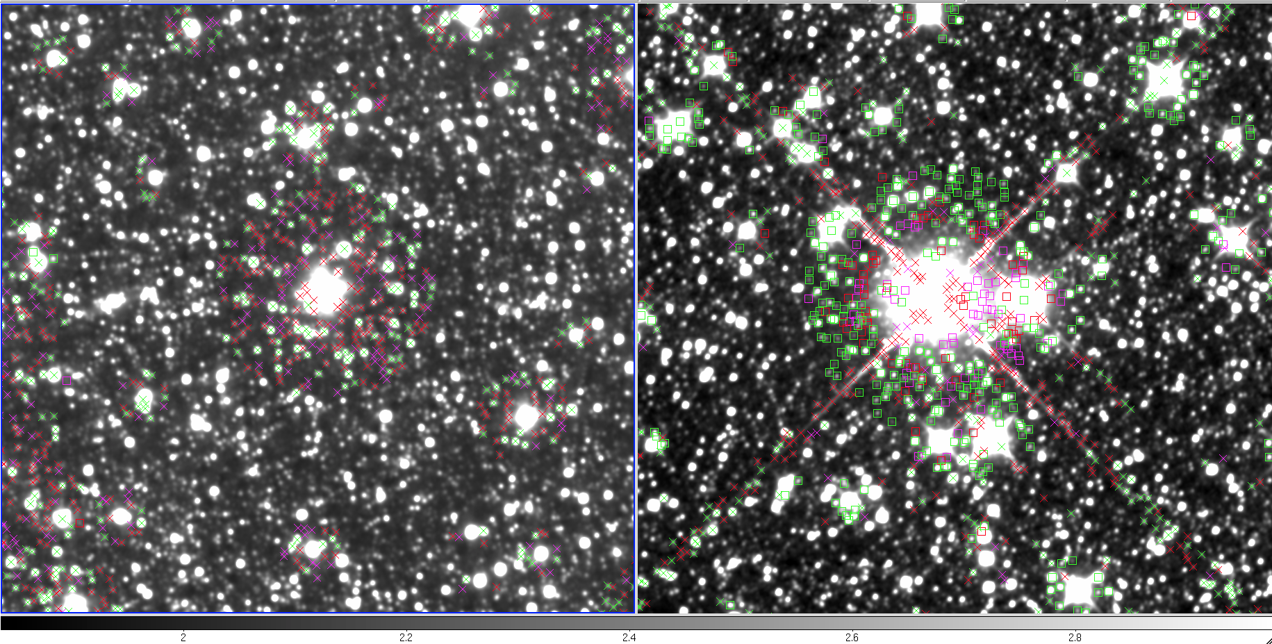Figure 21 - High-ecliptic-latitude effects on diffraction spikes

ii. Scattered-Light Halos

Bright sources are surrounded by a scattered-light "halo", essentially the outer portion of an object's point-spread function. This flux results in spurious extractions, and can, of course, also result in contaminated photometry for real nearby sources. Flagging of sources created or contaminated by halos is similar in the single-frame and atlas images; however, there are important differences outlined in the sections below.

ii.1 Single-frame Flagging

ii.1.a Halo Radius

To determine a function relating the halo radius, r_h, to the parent brightness, we plot the radius of the halo for several sources as measured from the altas coadds or frames vs. the magnitude of the parent source, m_p (Figure ??). The relation was determined to have the functional form,

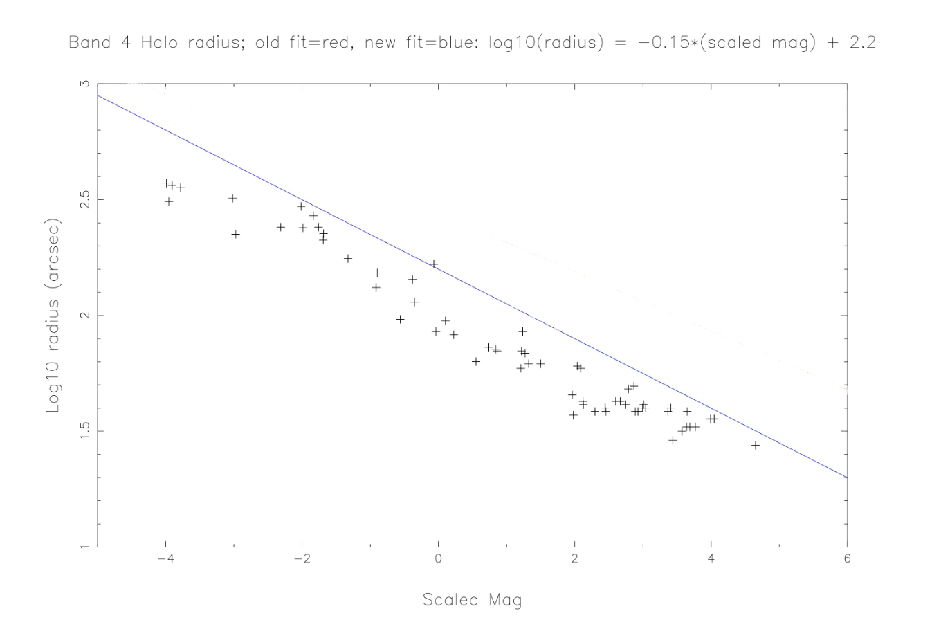Figure 22 - Example (band 4) of halo radius, rh, vs. parent magnitude for several sources in the atlas coadds. The blue line indicates the fit used.

We determine the optimum values for 'a' and 'b' in order to best predict a halo's radius. The fit overestimates the halo radius for the majority of magnitudes in order to ensure that all halo sources are flagged for all parent stars. The fitted parameter values are shown in Tables 11 and 12. These values were subsequently tuned using test runs of ARTID on numerous frames and atlas coadds.

ii.1.b Halo Real vs. Spurious Sources

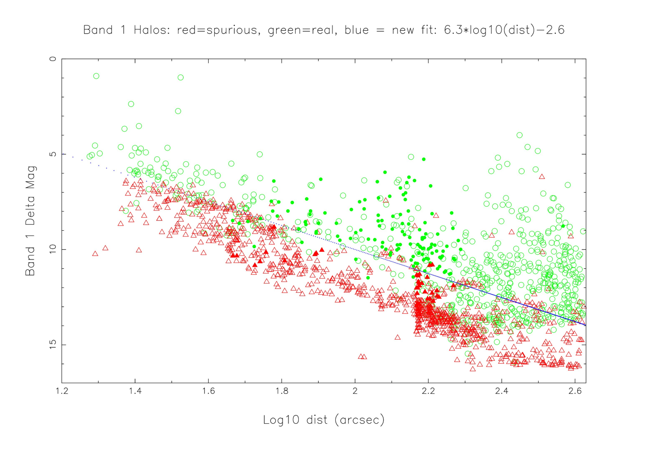
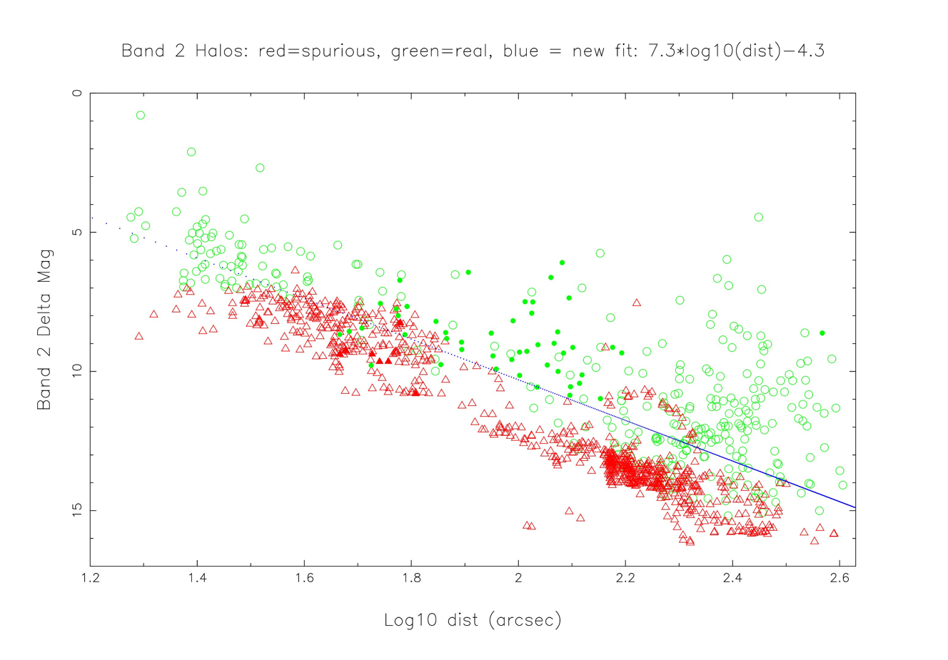
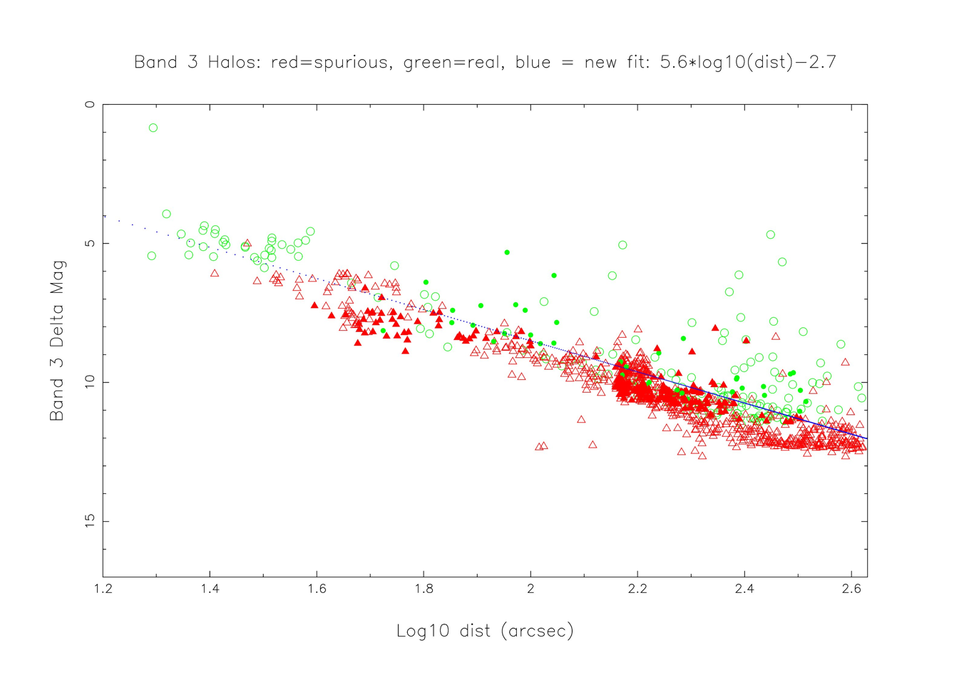
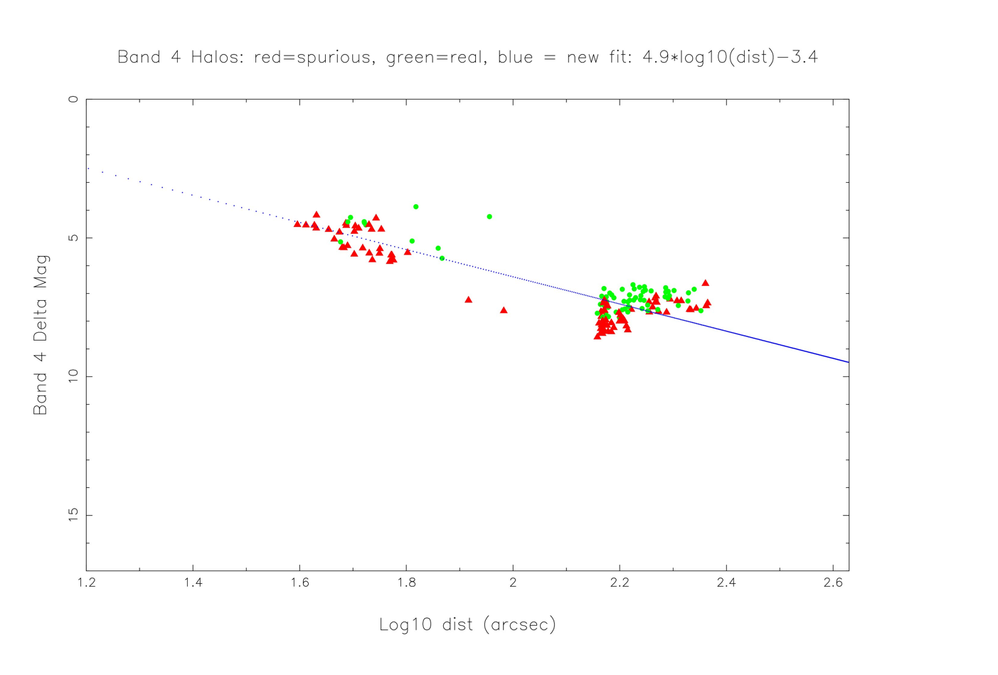
In order to differentiate spurious sources (those that are extracted from, and exist purely due to, the halo) from real sources that lie inside and are contaminated by the halo, we define a magnitude difference, Δm_{spur_h}. Consider an object which is extracted within the halo of the star to have a magnitude m_h. If m_h > m_p - m_{spur_h}, where m_p is the magnitude of the parent star, is considered a spurious source. Equivalently, if the object in the halo is bright enough that m_h < m_p - m_{spur_h}, it is considered a real and contaminated source. To determine optimal value of m_{spur_h}, as a function of the separation between the parent star and the halo source (d), we analyzed a number of sources from the atlas coadds and frames.

To begin, we selected a set of atlas tiles that contained bright stars (m > 5), separating bands 1 and 2 from bands 3 and 4 because the bright stars in bands 1 and 2 are not the same sources as those in bands 3 and 4. We examined the images for each band and tile in the set, and overlayed the complete source list in that band and the list of sources already marked as "halo" objects in that band. We next adjusted the image stretch so that we could see as many faint (and moderately bright) sources as possible in the image, so there was a clear difference between the diffuse halo emission and the background level; often we had to carefully find a balance between those two criteria.

For each of the brightest sources in the image, we selected the parent from the coadd [coadd_ID]-mfflag-3.tbl file or frame [scanframe_ID]-mfflag-1b.tbl file and marked it as such in a sorted copy of that file. We then examined each individual source in the halo region on the image and determined if it had the correct flag value. The method we used to determine the "correct" flag value was as objective as possible under the circumstances: we decided if the marked source is obviously a real source, i.e. it lies on top of a distinct local flux maximum, or obviously a false source, i.e. it lies on top of an area of confused, bright diffuse emission quite close to the parent or an area without any apparent source detection at all. If we felt we could not clearly determine the correct flag value, we ignored the source so the results would be as reliable as possible. This method results in a selection bias towards finding the real sources, since they are more obvious to the eye.

Below the parent source data, we added all the sources from the same file that were not marked as halo objects but which we believed should have been flagged, and appended the correct cc_flags value to the data ('H' or 'h' in the correct band's character). We did the same for the sources that were marked as halo objects but that we believed should not have been flagged, and appended the correct cc_flags value ('0' in the correct band's character). We added the sources that were marked as real or spurious halo sources ('h' or 'H', respectively) but which we thought should be marked as the opposite type, and again appended the correct cc_flags value to the data.And finally, we added some sources with flags that we agreed were correct.

We performed this analysis for as many parents in each image as possible, in order to get as large a range of parent magnitudes as possible. However, we concentrated on the brightest parents because the algorithm differentiating between the spurious and real halo sources should not depend on the parent magnitude; it only depends on the band, the distance between the parent and halo source, and the magnitude difference between the same.

After gathering all the results from this analysis, we ran them through a program that calculated the distance and magnitude differences between each parent and its corresponding halo sources. We then performed fits to this data, deriving a functional form for the relation:

Where 'a' and 'c' are the derived parameters. using different marks for the real and spurious halo sources as determined by the procedure above. We then drew a line in the region of overlap between the real and spurious sources, approximately in the middle of the region. This means that at this boundary line, about half of the sources are real and half are spurious. The derived values of the parameters are shown in Tables 13 and 14.

In the following figures (23 through 26), the green circles in the plots indicate real halo sources, and the red triangles indicate spurious sources. The open vs. filled marks only indicate different sets of images that were examined at different times; both sets of images apparently follow the same relationship between Δm and log10(d).

Figure 23 - Δm (parent - source magnitude) vs. distance from parent, d, Band 1.	Figure 24 - Same as Figure 23, but for Band 2.
Figure 25 - Same as Figure 23, but for Band 3.	Figure 26 - Same as Figure 23, but for Band 4.

ii.1.c Background Level Dependence

A major addition to the flagging of halos in the All-Sky Release is the incorporation of background level dependence in the determination of halo sizes. It became clear in the flagging of halos for the Preliminary Data Release, that the model used to predict halo radii was over-simplified. One of the components missing from the Preliminary Release model was the dependence of halo size on the background level of the frame where the halo appeared. In frames with a high background level, halos were generally smaller, as the faint outer parts of the halo drop below the level of noise at a smaller distance from the parent star. Thus, where background levels are high (in the galactic plane, for example), the halo radii are significantly overestimated by the model, leading to gross overflagging.

In order to mitigate this effect, we incorporate background dependent scaling for halo radii. For frames with high background levels, halo radii are reduced by a multiplicative scale factor. In other words, the background corrected halo length, r_{h_bg}, is related to the original halo length, r_h by the relation:

Where 'B' is the background scaling factor, generally a value between 0 and 1. The dependence of 'B' on background level is determined empirically. For each band, we generated a series of composite source space images, in a manner similar to the procedure described above for determining the parent magnitude dependence of halo sizes. In this case, however, we binned the parents by background level of the frame (the frame's value of 'medint' is used as a proxy for background level), in addition to their magnitude. We then determine the radii in each medint and magnitude bin by inspection of the source space image.

The relation between B and log(medint) is well-fit by a line:

where 'c_bg' and 'd_bg' are the parameters to be determined. For single-frame flagging, we determined that only Bands 1 and 2 displayed a significant variation for halo length with respect to background level. Thus, the parameters for Bands 3 and 4 were set so that no background-dependent scaling was applied to the final halo length. We also set minimum and maximum possible values for B. Figure 27 shows an example fit for four bright objects in Band 1 from a single scan of data.

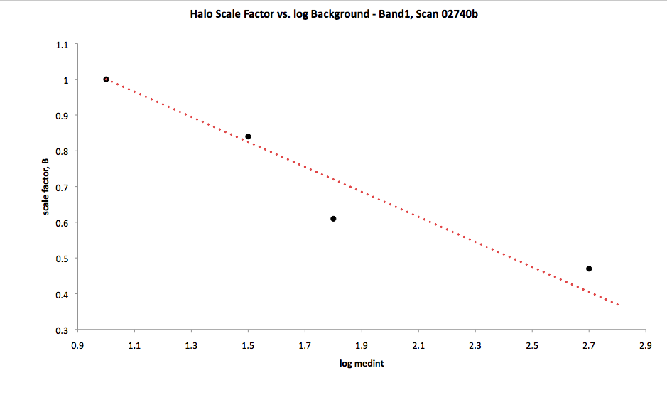Figure 27 - Example (Band 1) of background scaling factor, B, vs. background level, log(medint) for four sources from one scan, 02740b. The red dotted line indicates the fit used.

ii.2 Multiframe Flagging

Flagging for halos in the coadd images is essentially the same as in single-frame images. Parameters for halo radii, spurious thresholds and background scaling were determined in a manner similar to the single-frame characterization. Tables listing the multiframe parameter values are shown below.

Unlike single-frame flagging, Bands 3 and 4 show a dependence on halo size with respect to background level. Values for the background-dependent scaling are shown in Table 16, below.

There is one additional consideration during the flagging of scattered-light halos in the multiframe pipeline (which generates the final atlas images): the use of depth-of-coverage scaled magnitudes for parent stars. This addition is identical to the depth-of-coverage for diffraction spikes, and we refer the user to the appropriate section.

iii. Optical Ghosts

iii.1 Single-frame Images

Optical ghosts are the result of internal reflections in the optical path of the telescope. In the WISE images, ghosts manifest themselves as ring-like structures at a fixed position from a bright parent. Since, for a given band, ghosts always manifest themselves in the same position (direction and distance) relative to the center of a bright parent star flagging is performed using a purely positional approach. Sources are flagged inside a circular region located at a fixed distance and direction from the parent star's center. Although the ghosts themselves are not circular, a circular flagging region is a good first order approximation. The size of a ghost does not vary with the brightness of the parent star.

Parameters for ghosts include the radius of the circular region inside which sources are flagged (R_ghost). The positional offset from the center of the parent star, Δx and Δy, are also parameters. Additional parameters are m_{thr_o}, the parent star magnitude at which ghosts appear, and Δm_{spur_o}, the magnitude threshold used to differentiate spurious extractions on the ghosts from real sources whose photometry is contaminated by the ghost. The value of m_{thr_o} was determined by inspection of 50-100 of bright sources in single-frames over a range in brightness, and assessing the magnitude of the parent star at which ghosts no longer appear.

A source is determined to be spurious or real/contaminated using a constant threshold, Δm_{spur_o}. Given a magnitude of the source in question, m_s, and a parent-star magnitude of m_p, if m_s ≤ m_p + Δm_{spur_o}, then the source is flagged real and contaminated (i.e., if m_s > m_p + Δm_{spur_o}, the source is flagged as a spurious extraction). The value of Δm_{spur_o} is determined by selecting spurious extractions from ghosts in each band and, from their photometry, determining a difference in magnitude between the spurious extraction and parent star. The value of Δm_{spur_o} was chosen to be well lower than the average difference in magnitude to ensure that all spurious sources were flagged as such, with the side effect that some real sources are flagged as spurious. Both of these thresholds were tuned by test runs of ArtID on a large number of single frames, and inspection of flagging performance.

Examples of ghosts are shown below in Figure 28. Bright ghosts are most prevalent in Bands 2 and 3, with some in Band 4 as well. Band 1 sources do not generally have visible ghosts in single frames. Additionally, very bright objects in Band 3 have two ghosts, located in the negative y-direction, one below the other.

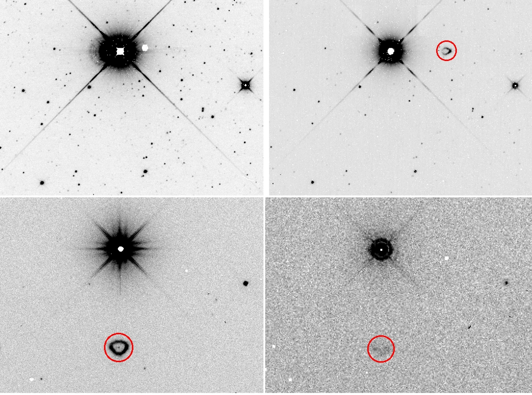Figure 28 - Examples of ghosts in the four WISE bands. The ghosts are indicated with a red circle and are seen in Bands 2 (upper right), 3 (lower left) and 4 (lower right). Ghosts are generally not visible in Band 1 single-frame images, but occasionally appear for extremely bright objects, in the same position relative to the parent star as Band 2.

For each band, the position of the ghost relative to the center of the parent is assessed, along with the radius of the circular region that is flagged. Table 17 shows values of Δx and Δy, R_ghost, m_{thr_o}, and Δm_{spur_o} for ghosts in each band. These parameters were initially determined by inspection of several tens of parent stars, over a range in brightness in each band, and were tuned using test runs of ArtID on single frames. Position and size parameters are given in single-frame pixels. Δm_{spur_o} is given in magnitudes.

iii.2 Multiframe Flagging

Since optical ghosts are always located in the same position relative to a bright parent star, they will appear, quite prominently, in coadded images. Optical ghosts in the multiframe version of ARTID are treated in much the same manner as single-frame flagging. The definition of the parameters remains the same as single-frame ghost flagging, however their values do change. For a description of the parameters, refer to single-frame ghost flagging. For example, values of m_{thr_o} due to use of depth-of-coverage scaled magnitudes for parent stars.

As with single-frame ghost flagging, parameters for ghosts include the radius of the circular region inside which sources are flagged (R_ghost). The positional offset from the center of the parent star, Δx and Δy, are also parameters. Additional parameters are m_{thr_o}, the parent star magnitude at which ghosts appear, and Δm_{spur_o}, the magnitude threshold used to differentiate spurious extractions on the ghosts from real sources whose photometry is contaminated by the ghost. The value of m_{thr_o} was determined by inspection of a 20-40 of bright sources and their ghosts taken from the atlas-type coadd test set (described in the Diffraction Spike section above), over a range in brightness. Values of Δm_{spur_o} were assessed in a manner similar to the single-frame determination, but using stars from the atlas coadd test set. The final values of the parameters are listed in Table 18, with positional offsets and R_ghost given in arcseconds (as opposed to single-frame pixels which were used in Table 17).

iv. Latents (Persistence)

iv.1 Single-frame Flagging

The following section contains information regarding the development and refinement of persistence (latent) artifact flagging. For the most recent information regarding changes to persistence flagging in the All-Sky Release please see the appropriate subsections for single-frame and multiframe flagging.

iv.1.a Short-term Latents: HgCdTe and Si:As arrays

There is an initial short-term latent that appears to be present at all signal levels above saturation for both the HgCdTe and Si:As arrays. The first frame after the illuminating frame has a latent present at < 0.1% (W1/W2) and 3% (W3/W4) of the peak flux density. The second frame has a 0.4% latent for W3/W4 only. The decay time is ~3 sec. The functional form of the decay of brightness in all bands is modeled as:

(Eq. 1)

where

F₀ = initial brightness of pixel in source

₀ = decay time = ~3 sec

B = pixel background brightness without source + bias

The short-term persistence behavior for the two types of detectors on WISE have similar decay times and strength; however, the morphology of the latent images is vastly different between HgCdTe (WISE bands 1 and 2) and Si:As (WISE bands 3 and 4). HgCdTe latent images are limited in size to the saturated region of the parent source. Thus, they are rarely more than a few pixels in extent. In contrast, Si:As short-term latent images are up to 100 arcsec in radius and are surrounded by an annular dark halo. The size of the pattern is the same for all saturated sources; however, the S/N of its appearance changes with parent source brightness.

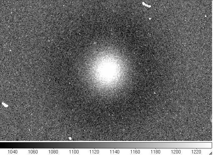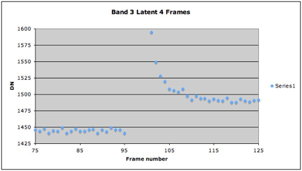
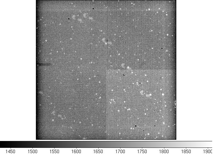
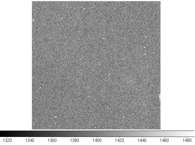
Figure 29 - Latents in WISE Band 3 introduced by a 95 Jy equivalent source. The displacement between the pixel values before frame 95 and after frame 115 is due to a long-term latent image of about 5% in gain. The exponential decay seen between frames 100 – 105 is due to a short-term latent.	Figure 30 - Long-term latent image in WISE band 4 shown by pixel value offsets introduced by a 32 Jy equivalent source produces an offset in the light curve of about 10% in gain.	Figure 31 - Si:As short-term latent image one frame after very bright W3 source. The entire pattern has a radius of approximately 100 arcsec although the parent source was unresolved.

iv.1.b Long-term Latents (Si:As arrays only)

Long term latent images appear with hard saturation of the detector. It is a gain effect that increases the response by about 10% in the pixels that exceed the threshold fluence. It is thus similar in extent to the HgCdTe short-term latent. The strength of the latent does not seem to correlate in an obvious way with the brightness of the initial source between 3 and 320 Jy. It is very similar in strength over an order of magnitude in illuminating source flux density. There is no obvious decay in strength of this latent during the 12 hours between anneals, although there is substantial decrease in their strength by 24 hours following emplacement. These latents are completely eliminated by 15K anneal heating of the arrays. Because of the multiplicative correction by dynacal in v4 (the all-sky data release), the long-term latents (which are response artifacts) do not appear as spurious sources in the single-frame or multiframe products. Due to this correction, the long term Si:As latents should not contaminate pixel photometry on frames more than 10 exposures downstream of the original illumination event.

Figure 32 - "Raw" (Level 0) WISE band 3 image showing long-term latents (bright splotches).	Figure 33 - Preliminary release single frame processing of same W3 image as in Figure Latent4. Long-term latents are mitigated through additive correction to frame.	Figure 34 - Mask file for Figure Latent5 image. Long-term latents show up as contiguous sets of "transient" pixels in the mask file. These pixels are excluded from source extraction in Level 1b and coaddition in Level 3.

At flux densities of several thousand Jy, the long-term latent undergoes a qualitative change in character from a positive to a negative gain effect. The dark latent depresses the value of the background by up to 5% in the ground tests. However, over a few hour timescale, dark latents evolve into long-term bright latents. These latents are completely removed by a 15 K anneal. In practice, most of the "dark latents" seen on the Level 1b images are due to overcorrection by the Dynacal algorithm.

iv.1.c Treatment of Latents by Single-frame WISE Pipeline

In the WISE pipeline, short-term latents are flagged using a predictive model. Sources brighter than a band-dependent magnitude threshold are placed in a latent parent database. The positions of these sources on the array are then tracked on subsequent frames as being potential latent image sites.  Table 19 shows the brightness thresholds per band used for determining membership in the latent parent database in the all-sky data release.

iv.1.d Changes in the All-Sky Data Release

There is a substantial change in triggering the cc_flag for latents in the all-sky release relative to the implementation in the preliminary release. In the preliminary release, circular regions of fixed size were flagged for latent parents of all brightnesses. However, in the all-sky release, the circular radius of pixels flagged for the presence of latents is given by a predictive model. The model is similar for all four bands; however, the parameters differ from band to band. The algorithm is of the form:

In the V4 WISE single-frame pipeline, sources falling within this radius from the detector position of  latent parents are flagged as artifacts due to the likelihood of their being spurious detections of the latent image ("P") or having photometry which is contaminated by presence of a latent image ("p"). The difference in magnitude between the latent parent source and a spurious artifact detection is controlled by the parameter Δm_spur. These parameters, as well as the decay time for short-term latents per band are listed in Table 3. For WISE bands 1 and 2, the model defaults to a fixed radius of 3 pixels when the brightness exceeds values of 1.0 and 0.0 respectively. In the case of short-term latents for bands 3 and 4, the radius of latent pixel flagging is also fixed for bright sources (magnitudes less than -1.0 and -2.0 for W1 and W2 respectively). For sources brighter than these magnitudes, the size of the region with latent flagging defaults to 50 pixels for W3 and 25 pixels for W4. In addition, for Si:As images there is also an outer annulus around the inner bright latent where sources are flagged as "contaminated" (symbol "p") as they may be depressed in response relative to sources falling outside this region. The outer radius is fixed at 100 pixels for W3 and 50 pixels for W4.

Since the zodiacal background emission varies markedly in the W3 and W4 wavelength regimes, the size of the region affected by latents also varies. The radius of the inner zone affected by Si:As latent images is scaled by the mode of the image background (MODEINT in the image header) in the following form:

latent_radius_scaled = latent radius * scale background/MODEINT.

The scale background per band is listed in Table 3.

For short-term latents, the latent flagging happens on frames immediately after the parent illumination event and ceases at the point where the decay model predicts the latent will have decayed below the S/N = 5 sensitivity level for a single frame. The characteristic decay time varies from band to band.

The WISE all-sky data release is significantly different from the preliminary data release in that a multiplicative (delta-flat) correction has been applied for long-term latent images. Thus, these artifacts are rarely seen in the all-sky single frames, although the infrastructure remains to flag dynasky resistent ("T" and "t") latents. For these long-term Si:As latents, the position occupied by the latent parent continues to be flagged until the next detector anneal.

The cc-flag symbol for latents is "p" or "P" (Persistence). Note that long- and short-term latents are flagged identically by the WISE pipeline and can only be distinguished by examination of the images.

iv.1.e Position Dependence of W2 Latent

The strength and longevity of the short-term latents over most of the W2 array behaves as described above. However, for bright stars with a saturated core located within the region loosely defined by the (X,Y) pixel coordinates (900-1000, 550-650), W2 latents can be brighter and longer-lived than usual. To demonstrate this effect, in Figure 35 we show the star SW Pic and its subsequent latent images at several different pixel locations on the W2 array. The characteristics of the latents are similar across most of the array, the exceptions being in scans 02710a and 08700a, where SW Pic is located at (X,Y) location (953,566) and (990,596), respectively. In these two scans, the latents are much brighter than normal and persist in three or more of the trailing frames. Users are cautioned that these longer duration latents may not be properly flagged by ARTID.

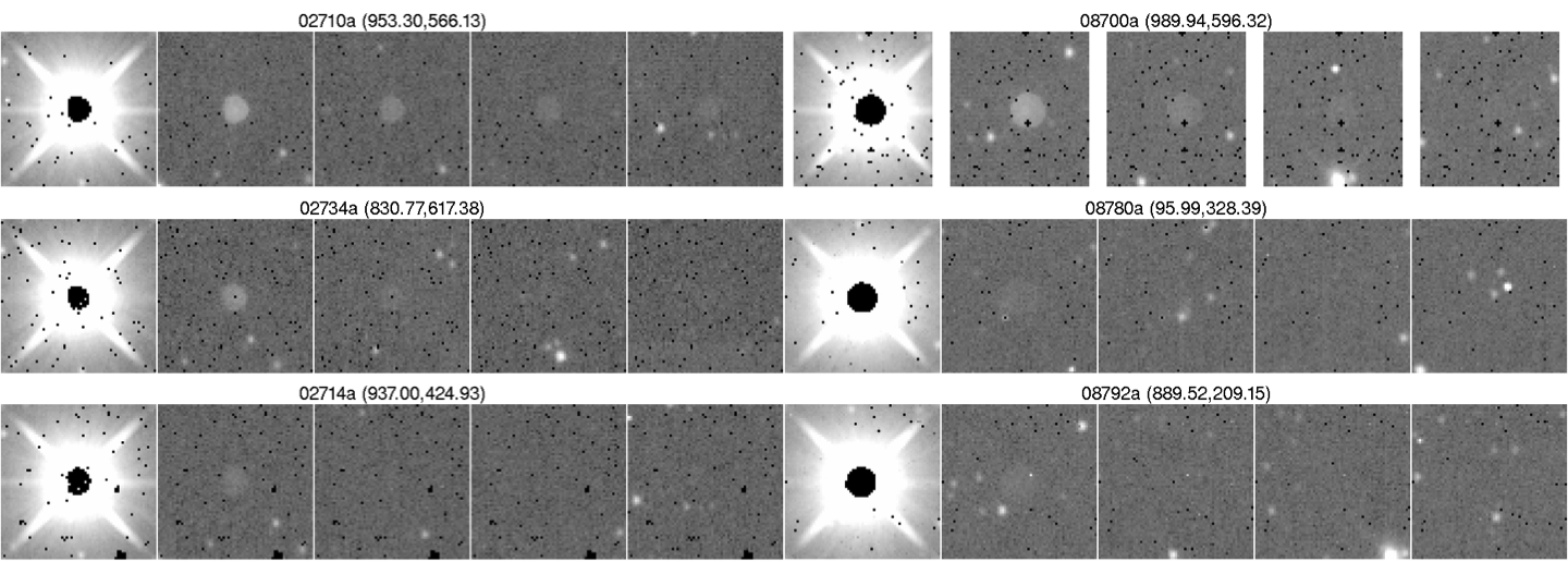Figure 35 - Examples of the position-dependent latent duration in W2 for the star SW Pic. The images are grouped in sets of 5 images showing SW Pic and the succeeding 4 frames to the right. The scanID and star's position on the array are indicated at the top of each set of images. The top row shows the star in the region that produces the longer duration short-term latent; the center and bottom rows show the star at another array position for comparison. The left column provides images from 4-band cryo whereas the right column is from 3-band cryo.

iv.2 Multiframe Flagging

In the V4 WISE coadd (MFF) pipeline, the radius for short-term latent flagging varies according to parent source brightness in all bands, and tile background for the Si:As arrays. Short-term latents, especially the large ones seen in the W3/W4 arrays, tend to add constructively in the coadded images and can be seen somewhat further downstream of their parent sources than in the single frames. However, in areas near the ecliptic poles, the outlier rejection algorithms tend to erode the actual latent images, although large swaths of sources will still be flagged as latents. In all cases, the images of sources suspected of being affected by latent images should be visually checked. Long-term latents are not flagged in the coadd pipeline. The sets of contiguous pixels in the V3.5 coverage images in which there were diminished coverage due to long-term latents have been eliminated in V4 due to the new delta-flat correction in Dynamic Calibration (see Section IV.4.a.viii of the Explanatory Supplement).

v. Glints

v.1 Single-frame Flagging

Glints are artifacts on single-frame images that occur when a bright source just off-frame produces reflected light which is imaged by the detector. Examples of different types of glints can be found in Figure 36. The names for the different types of glints ("feathers," "fans," and "needles") were chosen due to the morphology of the glints. "Feathers" appear in only Bands 1 and 2, "fans" appear only in Band 1, and "needles" appear in all bands. The upper panels in Figure 36 show Band 1 images with glints. One can also see diffraction spikes from the off-frame parents. The lower panel shows a Band 3 image with a glint produced by a parent located off-frame above the frame shown. One can also see the optical ghost and latent produced by the same parent. Glints in Band 2 display similar morphologies to Band 1, while Bands 3 and 4 show glints that are similar in nature, typically smaller than glints in Bands 1 and 2.

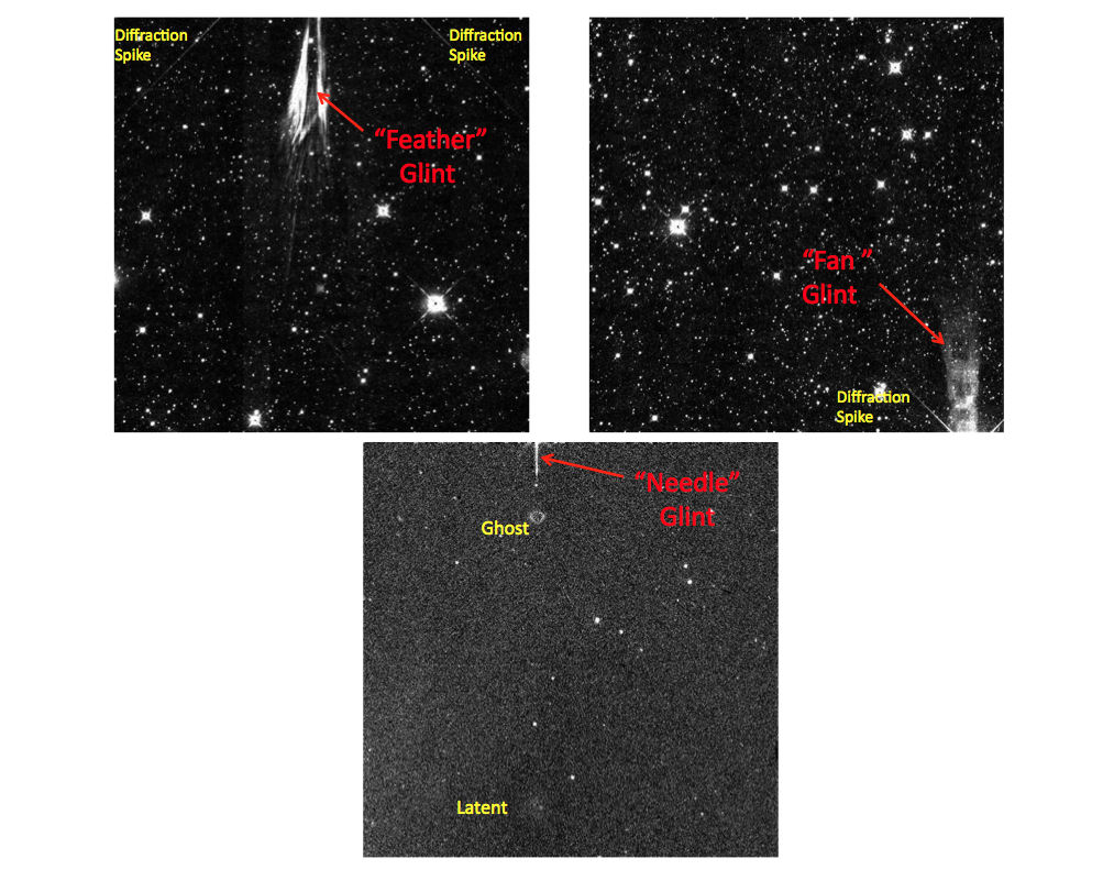Figure 36 - Examples of glints in the single-frame images. Upper-left- Band 1 "Feather" glint; Upper-right- Band 1 "Fan" glint; Lower- Band 3 "Needle" glint

The appearance of glints is somewhat predictable based upon the position of a bright source in the frame preceding and following the frame which shows a glint. Figure 37 shows how the appearance of glints are predicted, and how glints are flagged. The center row shows the frame in which two glints appear (the actual image is on the right, and a cartoon representation is on the left). The top row shows the preceding frame where one parent appears, while the bottom row shows the following frame where the parent of the second glint appears. As described above, glints are produced by bright parents located just outside the edges of the frame where the glints are seen. By examining about 140 glints in all bands, we determined that the locations of the glint-producing parents on the preceding and following frame were localized to a limited region. These regions are denoted by the pink shaded area and "Potential Parent Region" notation. When a bright star of a given magnitude appears in the potential parent region, it initiates flagging of all sources in the flagged region in the frame with the glints. The exact locations of the potential parent regions and the flagged regions were determined empirically using the aforementioned set of 140 glints. Tables 21 through 23 shows the parameters determined for three types of glints, "feathers," "fans," and "needles."

Due to the irregular morphology of most glints, as well as the existence of extensive "substructure" within each glint, we make no effort to differentiate between spurious and real extractions in the flagged regions. All sources within the flagged region are flagged with a cc_flags value of lower-case 'g'.

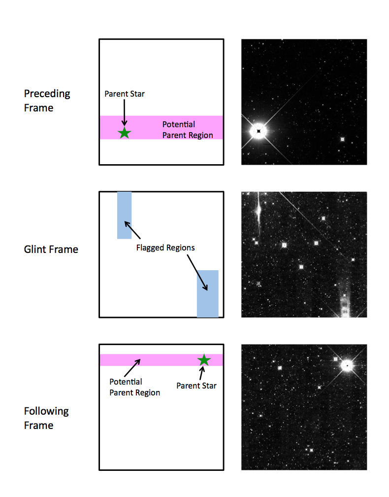Figure 37 - Characterization of Glint Parents and Flagging of Glints

In the following tables, the values of 'x' and 'y' describe the range of (x,y) pixel values located in the Potential Parent Region in the preceding and following frames (i.e., the parents are located above and below the glint frame, respectively). The value of 'FR' describes the length and width (in arcseconds) of the Flagged Region. The Flagged Region always begins at the edge of the frame directly below/above the parent in the preceding/following frame. The center of the Flagged Region is also offset a certain horizontal distance, FR_Δx (in arcseconds), from the center of the parent star. Finally, the brightness range (in mag) for the parents is given.

It should be noted that it is possible to have glints created by parents that are off-frame to the right and left of the glint frame. the numerous overlapping frames in the cross-scan direction that could contain a parent, these glints are not entirely predictable, and are not flagged.

v.2 Multiframe Glints

Glints are not flagged in multiframe processing. With the irregular morphologies and substructure, their varying "on-sky" positions, and the fact that the parents had to be in a very specific off-frame region to produce glints, it was anticipated that the outlier rejection in the frame coaddition process would remove glints from the final coadded images. It turns out that this was not case. In some cases, primarily for extremely bright parents, the glints appeared in enough single-frames, at similar enough positions that some glints appear in the atlas images, and are not flagged. Unfortunately, this leads to spurious sources in the All-sky Catalog. Thus, it is important to examine your sources in the images, to ensure that they are not spurious.

vi. The Bright Source List (BSL)

iv.1 The Bright Star List

Objects (usually stars) which cause most artifacts are saturated, and thus suffer a higher rate of measurement problems, including under-estimated fluxes and, in extreme cases, missed extractions. Since an extracted position and flux are required to model artifacts, remedial action was necessary to recover this information to optimize the completeness of artifact flagging. For this purpose the Bright Star List (BSL) was created.

The BSL is not a scientifically evaluated catalog but only for use in modeling artifacts. For this use, poor flux and position estimates are acceptable provided they are likely to be an improvement on what's available from WISE extractions whose artifacts are being modeled.

vi.2 BSL Generation

The BSL was constructed from a combination of WISE extractions from the pass 1 single exposure database, 2MASS Point Source Catalog (PSC) data, and IRAS Faint Source Catalog (FSC) data. BSL construction proceeded as follows:

• Search the pass 1 single exposure database for bright (w1,2,3,4mpro < 8,8,6,3) or saturated (w1,2,3,4sat > 0.1) detections.

  Each real object will have detections in multiple frames and thus the pass 1 data from this query will have many repeated measurements for each object. Combining these repeated measurements is discussed below.

• Match the returned WISE data to the 2MASS PSC.

  The BSL carries 2MASS magnitude data. 2MASS K_m is usually a good replacement magnitude for w1 and is often quite good for w2 as well. K_m will under-estimate the brightness of objects redder than main sequence stars for w1 and w2, but may still be a brighter, and thus more useful in artifact models, than the WISE magnitude estimate for some saturated objects.

• Collect groups of repeated observations of objects and select representative magnitudes and positions.

  A BSL entry was required to have multiple detections, from which the median magnitude was used. Positions came from the group member furthest away from the frame edge. Groups without 2MASS matches were rejected if group members are too spread out positionally, indicating the group was probably from a diffuse, extended object.

• Add unassociated bright 2MASS PSC sources.

  Because WISE pass 1 data failed to extract some very bright objects, the 2MASS PSC was searched for bright objects (K_m < 3) that matched no WISE BSL entries. These 2MASS objects were merged into the BSL.

• Associate to IRAS FSC

  IRAS FSC band 1 and 2 fluxes are carried in the BSL. For w3,4 WISE magnitudes which are poorly measured due to saturation, the FSC data provides better flux information than 2MASS if objects are redder than main sequence stars. Matching the FSC was facilitated by having FSC objects positionally identified with optical catalogs.

• Dynamically add bright SSOID apparitions for frame data.

  When the BSL is used in processing frame data, bright SSOID apparitions at the frame's epoch are added to the static BSL using modeled fluxes. This is not possible for Atlas tile data, which is multi-epoch.

vi.3 BSL Usage

• The BSL was used to replace magnitudes of saturated frame or tile extractions when a BSL magnitude is significantly brighter than the WISE extraction.

  Any of the WISE pass 1, 2MASS PSC, or IRAS FSC fluxes could be used to replace w1,2,3,4mpro values. These replacement magnitudes were used only for artifact modeling. Using BSL magnitudes in these cases usually significantly improved the model's fidelity at the small and acceptable cost of occasional over-flagging.

• Add BSL entries to the latent parent database if not present in the extraction list (frames only).

  This allowed potential latent parents to be found even if not present among the WISE extractions due to saturation issues. This increases the completeness of latent image artifact flagging.

• Use BSL entries for modeling of out of frame or out of tile sources.

  Since artifact modeling starts with frame or Atlas tile extractions, but the artifacts themselves could come from source outside the frame or tile, adding BSL entries for external sources was necessary to improve the completeness of artifact flagging. In the most dramatic cases, the BSL allowed for flagging diffraction spikes from sources several degrees off-frame or off-tile.

CAUTIONARY NOTES

1. If possible, examine all your sources by eye on the actual images. There are unflagged artifacts, as it is not possible to perfectly flag every single affected source.


2. For the cleanest possible search results (with respect to artifacts), we recommend requiring cc_flags = '0000' in your catalog searches. However, as noted above, there are unflagged artifacts, so examine your images.


3. Above we describe a method of accounting for variable depth-of-coverage in artifact flagging; we refer to this as parent magnitude scaling. This method has deficiencies in cases with low (< ∼10 frames) coverage or very high coverage (> ∼100 frames).
At low coverages, the scaling often underestimates the lengths of spikes and sizes of halos. Thus, when your searches are within a few degrees of the ecliptic plane, make sure to examine the images to ensure that your sources are not spurious extractions on diffraction spikes or halos. At the other extreme (near the ecliptic poles), spike lengths are often overestimated despite the inclusion of high-elat scaling. If your searches are within a few degrees of the ecliptic poles, you may want to allow lower-case (contaminated) flags for diffraction spikes and halos.


4. In the galactic plane, artifacts are often overflagged, due to the high background level in all bands. Our background scaling procedure somewhat mitigates this effect, but does not do a perfect job for the highest background levels. You may wish to allow contaminated (lower-case) flags for all artifacts if your search is within a degree or two of the galactic plane.


5. Treatment of near-ecliptic-pole diffraction spike lengths is NOT ideal, and does not completely account for shortening of diffraction spikes in this region. Spikes can be significantly overflagged within a few degrees of the ecliptic pole.


6. Large (> 1 arcmin) fuzzy bright objects surrounded by dark rings in the Si:As image data should always be presumed to be short-term latents from a bright source on a previous image. Although the size of the flagged region varies with parent and background brightness in the all-sky catalog, the algorithm is tuned for point sources only. Resolved, saturated nebulae will certainly cause a larger region to be affected on subsequent images than the automated pipeline will flag for latents. In addition, W1 and W2 latents, while small, are underflagged for very bright sources which saturate regions larger than 6 pixels in diameter. These appear as a clump of equally bright pixels on a frame following one with a saturated source on the same pixels. The best way to confirm that a source is affected by a latent is to look at the image and several preceding images.


7. Glints appear, but are not flagged in the multiframe pipeline (which produces the atlas images and catalog). Examine your images, especially when your sources are known to be near bright objects!


8. Glints appearing on the cross-scan sides of single-frames are not flagged.


9. As noted above, glint flags are always lower-case. If your source has a 'g' flag, inspect the source on the image to make sure it is not a spurious extraction.
   
10. In rare cases, a source may be bright enough that it produces a ghost which has a latent. These latents are not flagged. This occurrence is most common in Band 3


11. In the case of very bright objects, the Band 3 images can sometimes show a vertical "bleed" from the source. Although these artifacts look like diffraction spikes, they are not flagged.

Last update: 2016 February 24