


WPHOT is designed to perform the source position and flux characterization step associated with each of the three stages of source extraction during pipeline processing (single-frame, single-epoch 4-band frameset, and final multi-frame coadd stage). The characterization is based on an input list of source candidate positions produced by the source detection module, MDET, using a detection algorithm which makes use of the data at all bands simultaneously (additional details are given in Marsh & Jarrett (2011)).
Since the majority of sources detected by WISE are expected to be spatially unresolved, the optimal approach for source characterization involves profile-fitting photometry (WPRO). Profile-fitting is our primary method of flux estimation—it gives the best results for the majority (i.e., the fainter) sources, handles PSF variations and masked pixels in an optimal fashion, and extends the dynamic range for bright sources well into the saturated regime.
Just as with the detection step, profile-fitting is carried out using the data from all bands simultaneously. The advantages of simultaneous multiband extraction are:
The multiband estimation process represents a departure from the traditional procedure, employed in such software packages as DAOPHOT (Stetson 1987) and SExtractor (Bertin & Arnouts 1996), in which detection and characterization are carried out one band at a time. Another motivation for developing new source extraction algorithms is that currently available packages operate on a single regularly-sampled image rather than a set of dithered images. The procedures employed in MDET and WPHOT are optimized for the latter case.
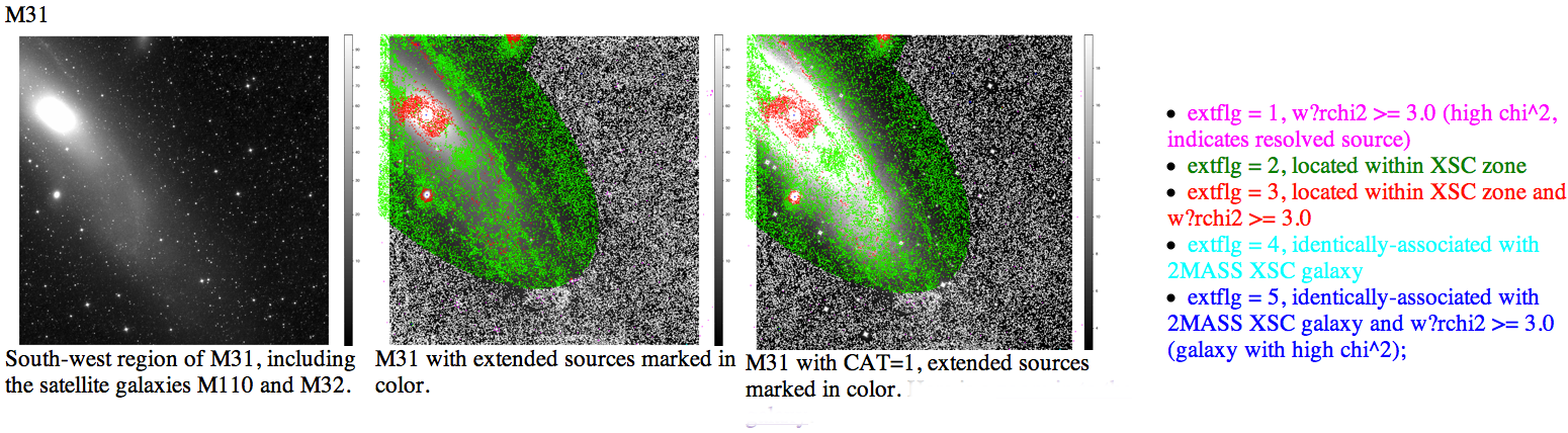
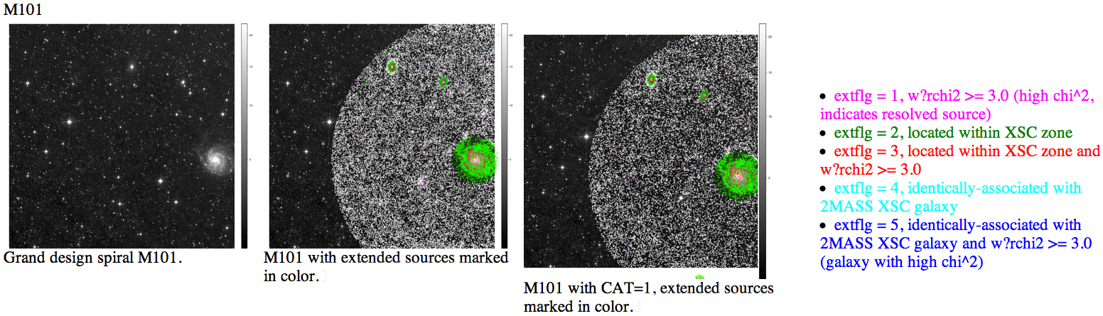
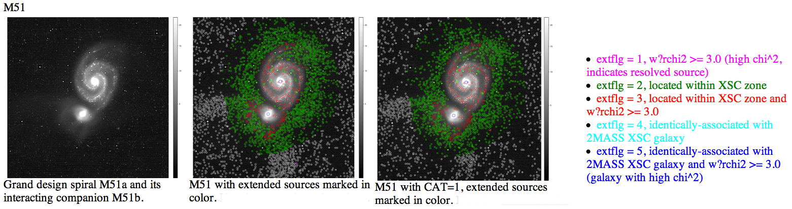
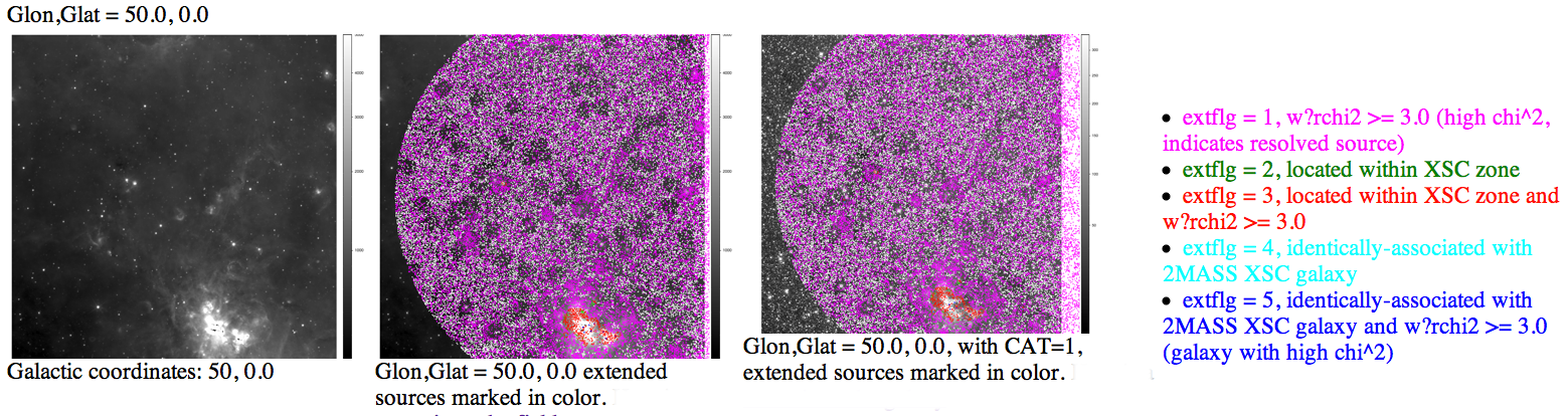
Since the majority of sources are unresolved, the profile-fitted flux represents our best estimate in most cases. For extended sources (one indicator of which is an elevated reduced chi squared value), an aperture flux should be used instead. Therefore, in addition to profile-fitting photometry, WPHOT includes a simple aperture photometry system (WAPPco) that employs circular apertures to characterize the integrated flux and "curve-of-growth" of point sources as measured in the co-added images. Those sources that are within close proximity to a 2MASS XSC (galaxy) are further characterized using an elliptical aperture derived from the 2MASS XSC.
 |
| Figure 1 - WPHOT Overview Flow Chart |
The compromise solution is to break the large co-add "footprint" into a smaller pieces, processing each piece separately. The cost is i/o overhead from reading in the frames multiple times, once for each grid piece. An example of a 3x3 divided footprint is shown in the diagram; a savings in memory load of nearly 50% is possible with such a gridding. The optical grid configuration, balancing run-time and memory usage is found to be 5x5.
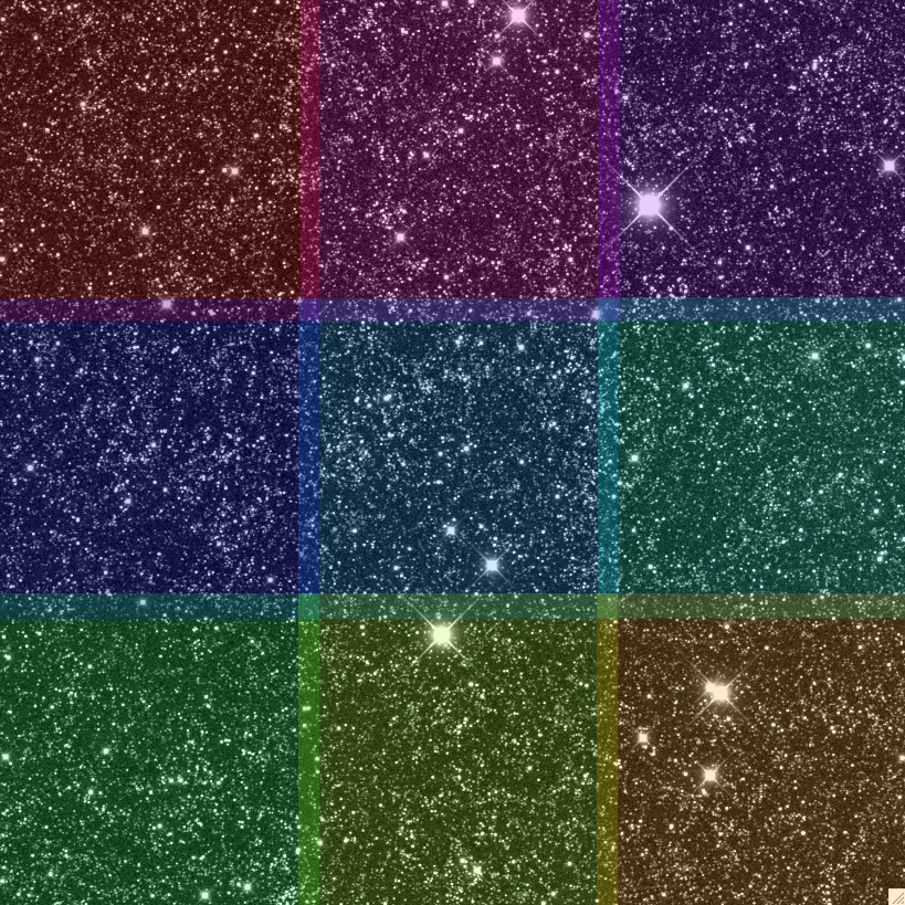 |
Figure 2 - WISE W1 co-add image, 4095x4095 pixels. The field has been divided into 3x3 pieces, thus reducing each piece to 1365 coadd pixels, or 683 frame pixels. A memory reduction of 45% is realized with this case. A small amount of overlap is needed to guarantee full processing coverage near division edges. |
The basic algorithm steps follow from the Co-add "footprint" divided into NxM pieces with enough overlap to take into account spacecraft rotation (w/ respect to equatorial north) and minimum border tolerance for background and source flux estimage; each piece is processed separately as follows:
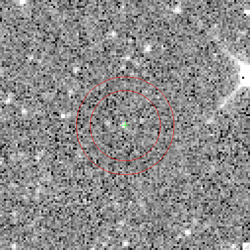
The local background is determined from the pixel value distribution within a circular annulus centered on the source MDET position. The source background, bλ and σ2bann, representing the local "sky" background level and its variance, are estimated from the number-weighted moment (or centroid) that comprises the pixel-distribution mode and its adjacent histogram neighbours. The mode, or most common binned histogram value, tends to be robust against the bright tail of the distribution that arises from stars and cosmic-ray (or hot) pixels in the annulus. Combining a weighted moment with a binned mode, or modified pixel-distribution mode mitigates limitations due to binning while exploiting the robust nature of mode estimation. The empirical uncertainty in the annulus local background (modified pixel-distribution mode), σ2bann, is also estimated from the histogram: where the standard deviation (about the mode) of all pixels on the faint side (or "left" side) of histogram represents the width of the distribution robust against the bright stellar tail; see figure for illustration.
The formal background error, or sigma in the mean, is derived from the the error propagation that follows the instrument characteristics and the noise model that is tracked by AWAIC and passed to on to WPHOT. With this noise model, the formal uncertainty in the background sky level is
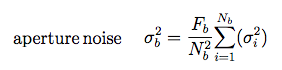 |
(Eq. 1) |
where Nb is the number of pixels in the annulus and
σi
is the measurement uncertainty for detector/frame pixel i,
and F_b is the correlation factor that is appropriate to the images
being measured (for single WISE frames, the factor is unity, and for co-adds it
ranges between 30 and 225, W1 to W4, respectively).
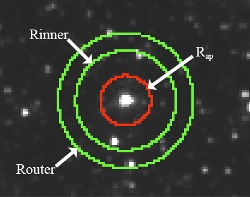 |
| Figure 3 - Parameters: standard aperture (red) and local background annulus (green). |
The formal background uncertainty is not sensitive to confusion noise that may be present in the aperture or annulus. It therefore requires a correction to account for any stellar crowding or confusion noise. A reasonable proxy to the total noise comes from the annulus background uncertainty, σ2bann. We therefore make the assumption that the confusion noise is the difference between the total noise in the annulus and the formal (Poisson) noise in the aperture:
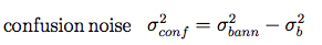 |
(Eq. 2) |
For most of the sky, the confusion noise term is zero or negligible in value, but for the Galactic Plane where stellar crowding is an important concern, the confusion noise term may be appreciable.
 |
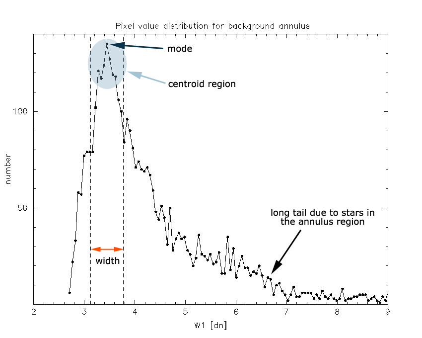 |
| Figure 4 - Example of a background annulus and its pixel value distribution (right panel). | Figure 5- The local background is estimated from the count-weighted 1st moment (or centroid) about the pixel distribution mode. The width of the histogram, representing the local background annulus uncertainty, is derived from the standard deviation of the pixel value distribution to the left-side of the mode. |
Choosing the optimal size for the annulus is an important consideration toward accurate photometry. The annulus must be large enough to avoid the influence of the point spread function and to minimize the Poisson component of the sky pixels (see equation below). On the other, it must also be small enough to represent the "local" sky value (that is to say, the fluctuations that are present in the aperture should be of similar amplitude in the annulus). Moreover, in order to accommodate the possibility of the source being a fuzzy galaxy, the annulus should extend beyond the size expected for most galaxies in the sky.
Consider what was done with 2MASS background estimation. For standard 2MASS point source photometry, the annulus that was used: R_inner = 14 arcsec, R_outer = 20 arcsec, with 2 arcsec pixels that translates to 160 pixels in the annulus. The 2MASS beam is about 2.5 arcsec, so R_inner is ~6x the FWHM. For the combined calibration fields, 2MASS used a larger annulus, 24 - 30 arcsec in size, or roughly ~10x the FWHM. For comparison, the standard calibration aperture for Spitzer-IRAC is 12 arcsec, and the annulus is 14.4 - 20 arcsec, which compared to the 2 arcsec beam is ~7 - 10x the FWHM.
For WISE, the FWHM=6 arcsec for the short channels, and so using 2MASS/IRAC as a guide, the inner radius would be ~40 - 50 arcsec (80 - 100 arcsec for WISE-4); with 2.75 arcsec pixels, that translates to R_inner ~ 15 - 18 pixels. For the width, using a similar area as the 2MASS/IRAC annulus, then R_outer ~ 19 pixels. Since that is a relatively thin aperture, subject to pixelization effects, it would be better to extend it to a width of 4 - 5 pixels, or R_outer = 20 - 22. Consequently, the adopted annulus for WISE point sources is: 50 - 70 arcsec (for all four bands), corresponding to 18-25 pixel radius in W1, W2, W3, and 9 to 13 pixels for W4. This setting is constrained by the W4 beam.
Local Background Output ParametersThe purpose of this step is to make a maximum likelihood estimate of the source position and the set of fluxes at the four wavelengths for each source candidate identified by the detection module MDET. The candidate source and its neighbors (i.e., adjacent candidates whose PSF responses overlap significantly with the primary candidate) are grouped into blends, and their parameters estimated simultaneously; this process is referred to as passive deblending, and is incorporated explicitly into the photometric measurement model. The critical distance for blend grouping is driven by the size of the PSF at the longest wavelength; neighbors separated from the source in question by less than twice the nominal FWHM at W4 (i.e., 24 arcsec) are included in the initial blend group. Not included, however, are those components whose initial estimates of aperture flux are more than 2.5 magnitudes fainter than the primary.
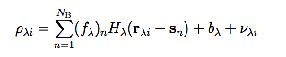
For a blend consisting of NB components, the measurement model used in profile fitting is:
 |
(Eq. 3) |
where ρλi is the observed value of the ith pixel at 2-d sky location rλi in the waveband denoted by subscript λ, sn is a 2-d vector representing the location of the nth blend component, fλn is the flux in the λth waveband, Hλ(r) is the PSF, bλ is the local background, estimated in an annulus surrounding the candidate position, and νλi is the noise, assumed to be a spatially and spectrally uncorrelated zero-mean Gaussian random process with variance σλi2.
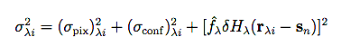
The latter quantity includes the various noise components in the error model and may be expressed as:
 |
(Eq. 4) |
where (σpix)λi represents the uncertainty in the pixel value due to instrumental effects; it is calculated by module ICAL, and includes the effects of Poisson noise, read noise, and flat-fielding error. Also, (σconf)λi represents the confusion noise, as defined by Eq. (2) above, and δHλ(r) represents the PSF uncertainty which must be scaled by the source flux, f^λ. The "hat" symbol (^) over the latter quantity denotes an estimated value. Our best estimate prior to the profile fitting is the aperture flux; we follow this with a second iteration based on the profile-fitted flux from the first iteration.
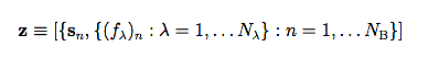
The set of unknowns in the estimation process can be represented by an np-dimensional parameter vector, z, defined as:
 |
(Eq. 5) |
where Nλ represents the number of wavebands, and the number of unknowns is given by np = NB(Nλ + 2).
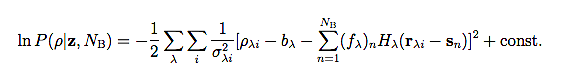
The solution procedure is to maximize the conditional probability P(ρ|z,NB) with respect to z, where:
 |
(Eq. 6) |
in which the summation over i is for all pixels within a predefined "fitting radius", rfit, of the candidate source location. Pixels which are flagged as "bad," due to effects such as saturation and cosmic ray hits, are excluded from the solution. We normally set rfit = 1.25 x FWHM, where the latter quantity represents the nominal FWHM of the PSF at the particular band, equal to 6, 6, 6, and 12 arcsec in bands W1 through W4, respectively. However, in the case of saturated stars, we set rfit = max(2rsat, 1.25xFWHM), where rsat is the effective radius of the saturated core of the bright star, calculated by the MDET module.
The quality of the fit is then evaluated using the reduced chi squared, given by:
 |
(Eq. 7) |
where Nobs represents the total number of pixel values used in the solution.
Before proceeding further, the blend group is first examined to check for redundant components, i.e., those components which can be removed without an increase in χν2. Thus the final value of NB can, in some cases, be less than the initial value defined above.
If χν2 ~ 1, the fit is regarded as satisfactory.
However, if χν2
is larger than a critical value,
(χν2)crit,
or if the reduced chi squared for an
individual band (denoted
(χν2)λ)
exceeds a related threshold,
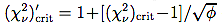 (where
φ is the relative number of degrees of freedom of the single-band fit
with respect to the multiband fit),
then we consider that the source model has not satisfactorily reproduced the
observed data. We then examine the hypothesis that the true intensity
distribution involves additional point source components. In this procedure,
referred to as active deblending, we successively add more source
components (thereby increasing NB) until either
χν2 <
(χν2)crit
or else the blend number
reaches a predefined limit, (NB)max, at which
point we conclude that a model consisting of a few point sources
is not consistent with the observations. For reasons of computational speed,
we allow at most 1 extra component to be added via active deblending.
(where
φ is the relative number of degrees of freedom of the single-band fit
with respect to the multiband fit),
then we consider that the source model has not satisfactorily reproduced the
observed data. We then examine the hypothesis that the true intensity
distribution involves additional point source components. In this procedure,
referred to as active deblending, we successively add more source
components (thereby increasing NB) until either
χν2 <
(χν2)crit
or else the blend number
reaches a predefined limit, (NB)max, at which
point we conclude that a model consisting of a few point sources
is not consistent with the observations. For reasons of computational speed,
we allow at most 1 extra component to be added via active deblending.
At each iteration of the active deblending procedure, the mechanism for adding a new source component is as follows:
We used (χν2)crit values of 1.5 and 3.0 for the "trigger" and final acceptance values, respectively, and set (Δχν2)min = 0.25.
The overall profile-fitting photometry procedure is illustrated by the flow chart in Figure 6; the active deblending procedure is contained within the blue dashed rectangular box. Active deblending is required for sources whose separation is less than 1.3 times the FWHM of the PSF at a given band, since this is the critical distance at which the detector can resolve neighboring sources.
 |
| Figure 6 - WPRO Flow Chart |
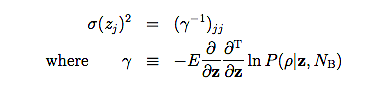
When a satisfactory solution has been obtained, the uncertainties in the estimated parameters (position and fluxes) are obtained using:
 |
(Eq. 8)
|
in which E is the expectation operator and T denotes transpose.
In cases for which χν2 is large (e.g. >2), the quoted flux uncertainty may not accurately reflect the true uncertainty because a poor profile fit indicates a violation of the statistical assumptions associated with the measurement model. There is, in fact, no direct correlation between the χν2 values and the quoted measurement uncertainties since the latter are determined from an a priori error model (albeit with some data-dependent parameters) that does not incorporate the a posteriori information regarding the quality of the fit. In most cases, a large value of χν2 indicates the presence of confusion with nearby sources or contamination by image artifacts or masked pixels.
The way in which the overall estimation procedure is implemented is that we start with the brightest source in the candidate list and estimate its parameters as above. We then proceed as follows:
We then repeat the procedure for the next brightest candidate, and so on until the MDET candidate list is exhausted.
Each PSF in the library represents an average over a focal-plane segment of width WP, over which we approximate the PSF as locally isoplanatic. The driver for WP is the Functional Requirement of at least 7% flux accuracy for an unsaturated source with SNR > 100. Our 9x9 subdivision of the focal plane exceeds this requirement by typically better than a factor of 4. We now discuss in detail the procedure used for PSF estimation in each focal-plane segment.
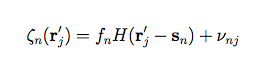
The measurement model for the PSF is then:
 |
(Eq. 10) |
where sn is the location of the nth star in the segment. The origin of the coordinate system for the PSF image is defined to be at the star location.
The noise, νnj, is assumed to be an uncorrelated Gaussian random process for which
 |
(Eq. 11) |
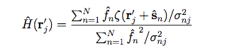
From the set of star images, we can make a maximum likelihood estimate of the PSF using:
 |
(Eq. 12) |
where f^n and s^n represent the estimated flux and position, respectively, of the nth star. For bright stars, an accurate flux estimate can be obtained via aperture photometry.
The source position sn is estimated by adjusting the positional offset of the star image for maximum correlation with respect to a nominal starting PSF, H0(r'), for which we used a theoretical form based on optical simulations. The estimation is accomplished by numerical minimization, with respect to sn, of:
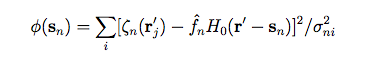 |
(Eq. 13) |
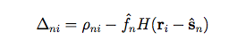 |
(Eq. 14) |
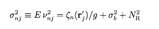
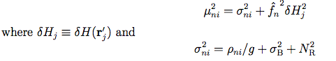
We model Δni as a zero-mean Gaussian random process with variance
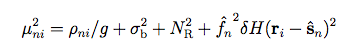 |
(Eq. 15) |
where δH(r) represents the PSF uncertainty at offset r from the PSF origin; g and NR represent the gain and read noise, respectively.
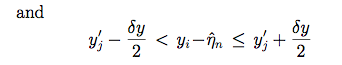
Suppose that the position (ri - sn) falls within the jth pixel on the grid used to represent the PSF, i.e.,
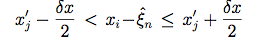 |
(Eq. 16) |
 |
(Eq. 17) |
where (x'j, y'j) represent the components of r'j, (ξn, ηn) represent the components of sn, and δx, δy represent the sampling intervals of the PSF grid in the x and y directions, respectively.
Then:
 |
(Eq. 18) |
Thus the probability density of the set of local data residuals, Δ, conditioned on δHj, is given by:
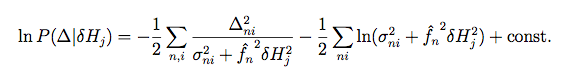 |
(Eq. 20) |
where the summations are over all n, i which satisfy Equations 16 and 17 for a given j.
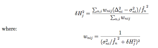
This expression is maximized when:
 |
(Eq. 21)
|
Since δHj is present on both sides of Equation 20, an iterative solution is required. Convergence is rapid, however, and a single iteration suffices.
For each focal plane segment:
1. Locate all stars above a given flux threshold for the particular band.
2. Estimate PSF and its uncertainty using Equations 12 and 21.
3. For each individual star, examine the quality of its profile fit by evaluating χν2 using Equation 7.
4. List any stars for which χν2 exceeds a predefined threshold (~ 2); discard the star with the highest χν2
5. Iterate from step 2 until all all remaining stars used in the PSF estimation have acceptable profile fits.
The PSFs and their corresponding uncertainty images, as used for the Preliminary Release, were generated one band at a time using the procedure described above. Candidate frames were selected from all scans between 01601a (by which time improved astrometry had been implemented) and 01751a. Initial frame selection was made by searching source detection tables for bright unsaturated stars, requiring SNR of at least 30 in the case of W4. This yielded 1028 candidate framesets. The W1 images were then visually examined to remove those images with obvious tracking problems (elongated images), high cosmic ray fluxes, highly crowded fields in the Galactic plane, structured backgrounds (e.g. nebulae), very bright stars saturating large areas of the array, and scattered moonlight. This selection process left 888 candidate framesets. The practical limit on the number frames that WPSFGEN can process at once is ~500, so another 300 framesets were removed by randomly rejecting framesets which had only one band four detection with W4SNR > 30. The final list of 484 frames provided 68749 unique sources with SNR > 100.
For bands W1-W3, PSFs were generated in 9x9 grids over the focal plane. Because of the relative scacity of bright stars in W4, a 5x5 grid was generated, and interpolated between adjacent PSFs to form a 9x9 grid. The following is aset of pseudocolor representations of the PSFs using a linear intensity scale, clipped at 60% of peak; the width of the field of view is 43.5 arcsec for W1-W3 and 87 arcsec for W4:
 |
 |
 |
 |
| Figure 7 - WISE PSFs | |||
Compressed tar files containing the grid of FITS PSF images
shown in Figure 7 for each of the bands are available by clicking on the
links below:
See the README file for a description of the contents of the files.
Profiles through the central PSF in the 9x9 array in each band are shown in Figure 8. The major axis has been defined as that for which the FWHM is maximized, and the minor axis is perpendicular to that.

|
| Figure 8 - PSF profiles through major axes (solid lines) and minor axes (dashed lines). |
The major and minor axes and position angles of major axes of the central PSFs are then as follows:
| Band | Major Axis FWHM [arcsec] |
Minor Axis FWHM [arcsec] |
Major Axis PA [deg] |
|---|---|---|---|
| W1 | 6.08 | 5.60 | 3 |
| W2 | 6.84 | 6.12 | 15 |
| W3 | 7.36 | 6.08 | 6 |
| W4 | 11.99 | 11.65 | 0 |
Noise pixel estimates can be found in IV.6.c.i.
As discussed above, WPRO increases the fitting radius for bright saturated stars, making use of the surrounding annulus of unsaturated pixels. For very bright stars, the saturation region can be larger than the PSF size itself, leaving no usable pixels within the fitting radius. This is not a problem in W4, but occurs frequently in W1 - W3. For this reason, we have fitted extended wings to the PSFs in the latter three bands. This was accomplished by using the images of bright saturated stars at a large number of positions over the focal plane. There were, however, an insufficient number to determine the behavior of the PSF wings in all of the 9 x 9 subregions of the focal plane, so a single average PSF-wing image was derived for each of the three bands. This image was then used to extend the wings of each PSF in the 9 x 9 grid at that band. The field of view of the resulting augmented PSF images in W1 - W3 was 3.67 arcmin; this was sufficient to do photometry on even the brightest saturated stars. The resulting PSF images are shown in Figure 8a below. Corresponding uncertainty maps were derived from the residuals between the average PSF-wing images and the individual bright star images. The outer wings of the resulting PSFs are rather uncertain, and hence the brightest saturated stars have large uncertainties in their quoted magnitudes.
 |
 |
 |
|
| Figure 8a - Extended wings of WISE PSFs. Shown on a linear intensity scale, clipped at 0.1% of PSF peak. | |||
w?sat: The number of saturated pixels located within the photometric "fitting" region in the vicinity of the source, expressed as a fraction of the total number of pixels within that region. The saturated pixels themselves were excluded from the solution, as explained above.
w?frtr: The fraction of pixels within the fitting region which were flagged as bad pixel transients. These pixels were also excluded from the solution. Note: The w?frtr values are set to 0.0 in the All-Sky Release Source Catalog and Reject Table, and the 3-Band Cryo Source Working Database, so cannot be used to select (or deselect) entries in queries on those tables.
Multiple independent measurements allow assessment of time variability. WPRO extracts not only the composite flux for a source but also the individual measurements. The WISE pipeline applies some simple tests to assess significant excursions beyond mean values:
N of M refers to the number of S/N > 3-σ extractions relative to the total number of measurements for a source. Sources that are low S/N will have a low N/M fraction, and conversely high S/N sources should have a fraction that is unity. Those sources that are high S/N but exhibit a low N/M fraction may indicate measurement failures or source instability.
The distribution in individual measurements has a mean and standard deviation of the mean and population. Sources that are high S/N but exhibit a large standard deviation may indicate short-time scale variability or measurement failure.
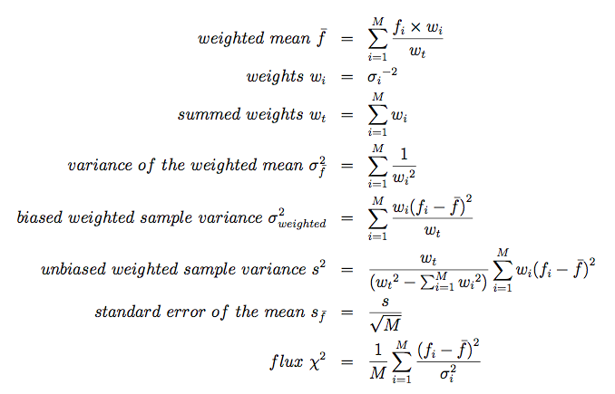 |
(Eq. 23)
|
The weighted mean, the unbiased weighted sample variance (re: population variance) and the standard error of the mean are reported. Comparison of population variance with composite WPRO flux variance may be used to assess time variability; see next section.
Repeatability Output Parameters
The WISE Catalog/Reject Table source records contain a variability flag, var_flg, that provides a measure of the probability that the flux of the object varied over the time spanned by the individual Single-exposure observations. This flag is evaluated by analyzing the distribution of the individual flux measurements of each source in each band, and the correlations between the bands. A detailed description of the algorithms used to define the var_flg values is given in IV.4.c.iii.6.
The Catalog/Reject Table also contains parameters related to the flux variations in each source, including factors that are used to determine the values of var_flg. These parameters include:
| Column Name | Format | Units | nulls | Description | |
|---|---|---|---|---|---|
| w?dmag | %5.3f | mag | yes | Difference between maximum and minimum magnitude of the source from all usable frames in band ?. Single-frame rchi2 values greater than 3.0 times the median are rejected. | |
| w?ndf | %6d | ---- | yes | Number of degrees of freedom in the flux variability chi-square in band ?. | |
| w?mlq | %4d | ---- | yes | Probability measure that the source flux is in band ?. The value is -log10(Q), where Q = 1-P(chi2). P is the cumulative distribution probability for flux[1]. The value is clipped at 9. | |
| w?mjdmin | %17.8f | day | yes | The minimum modified Julian Date (mJD) of the frames containing the source in band ?. | |
| w?mjdmax | %17.8f | day | yes | The maximum modified Julian Date (mJD) of the frames containing the source in band ?. | |
| w?mjdmean | %17.8f | day | yes | The mean modified Julian Date (mJD) of the frames containing the source in band ?. | |
| rho12 | %4d | percent | yes | The correlation coefficient between the W1 and W2 single-frame flux measurements. The value is a signed 2-digit integer, expressed as a percentage. Negative values indicate anticorrelation. | rho23 | %4d | percent | yes | The correlation coefficient between the W2 and W3 single-frame flux measurements. The value is a signed 2-digit integer, expressed as a percentage. Negative values indicate anticorrelation. | rho34 | %4d | percent | yes | The correlation coefficient between the W3 and W4 single-frame flux measurements. The value is a signed 2-digit integer, expressed as a percentage. Negative values indicate anticorrelation. | q12 | %4d | ---- | yes | Correlation significance between W1 and W2[2]. The value is -log10(Q2(rho12)), where Q2 is the two-tailed fraction of all cases expected to show at least this much apparent positive or negative correlation when in fact there is no correlation. The value is clipped at 9. | q23 | %4d | ---- | yes | Correlation significance between W2 and W3[2]. The value is -log10(Q2(rho23)), where Q2 is the two-tailed fraction of all cases expected to show at least this much apparent positive or negative correlation when in fact there is no correlation. The value is clipped at 9. | q34 | %4d | ---- | yes | Correlation significance between W3 and W4[2]. The value is -log10(Q2(rho34)), where Q2 is the two-tailed fraction of all cases expected to show at least this much apparent positive or negative correlation when in fact there is no correlation. The value is clipped at 9. |
| Notes: [1] The Q value is the fraction of all cases to be expected if the null hypothesis is true. The null hypothesis is that the flux is emitted by a non-variable astrophysical object. It may be false because the object is variable. It may also be false because the flux measurement is corrupted by artifacts such as cosmic rays, scattered light, etc. The smaller the Q value, the more implausible the null hypothesis, i.e., the more likely it is that the flux is either variable or corrupted or both. [2] When the number of measurements is large, the significance of correlation also tends to be large even though the correlations themselves may have a small magnitude. This is a typical manifestation of statistical significance increasing as the sample size increases; eventually the significant effect can be due to small correlated errors in background estimation or even roundoff errors. These effects tend to be small but become significant when there are enough observations of them. High flux correlation significance should be taken seriously only when the magnitude of the correlation is also fairly high. | |||||
It should be understood that the profile fitting system (WPRO) represents the most accurate flux estimation for point sources under most circumstances. The exceptions are when the source is high S/N (>> 50) but not saturated or when it is resolved with respect to the PSF. Circular aperture photometry provides a better flux estimation for both of these cases. If the source is associated with a 2MASS extended source, then WAPPco provides an elliptical aperture measurement designed to capture a larger fraction of the source flux as described below.
The basic flow of the WPHOT co-add photometry system WAPPco is illustrated in Figure 9. Fixed serves several purposes, including:
 |
| Figure 9 - System Flow Chart |
The primary functions of WAPPco are to carry out circular aperture photometry and local background estimation. It performs the initial (preliminary) flux measurements for source characterization by WPRO, and applies a full suite of circular aperture measurements on the co-added Atlas Images. The aperture mask is scanned for bad, saturated or fatal-flagged pixels, and the aperture flux is flagged accordingly. If nearby stars are detected within the aperture, the flag is set to indicate contamination. If the source is associated (in position) with a 2MASS XSC source, elliptical is carried out using an aperture based on the 2MASS extraction. Finally, if the source is suspected to be extended (e.g., poor χ2 value ), then it is flagged as such.
| bands | 1 | 2 | 3 | 4 | 5 | 6 | 7 | 8 | units |
| W1, W2, W3 | 5.50 | 8.25 | 11.00 | 13.75 | 16.50 | 19.25 | 22.00 | 24.75 | arcsec |
| W4 | 11.00 | 16.50 | 22.00 | 27.50 | 33.00 | 38.50 | 44.00 | 49.50 | arcsec |
| W1 | W2 | W3 | W4 |
| [mag] | [mag] | [mag] | [mag] |
| 0.222 | 0.280 | 0.665 | 0.616 |
There are several functions of the WAPPco system, multiple aperture photometry is the primary function of the WAPPco system. The standard aperture is used to measure the source brightness in a small aperture, which is then corrected so that it recovers the "total" flux of the source, thus matching the PSF-measured flux of the source. A set of nested circular apertures centered on the source (as determined by WPRO) provides the "curve of growth" for a source. The aperture sizes range from the smallest APMIN (5.5 arcsec, or 4 co-added pixels) to the largest APMAX (24.75 arcsec, or 18 co-added pixels), which is constrained by the background annulus. The photometry is carried out using code, developed by 2MASS, that is adapted for WISE images. It includes fractional pixel computations and the ability to use non-circular (elliptical) apertures that are deployed for measurements of 2MASS XSC galaxies.
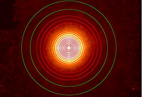 |
| Figure 10 - Set of nested circular apertures (red) and background annulus (green). |
Formal aperture and error model measurements
(see also II.3.f):
 |
(Eq. 31)
|
where G is the gain (electrons per DN), Nap is the number of pixels in the circular aperture of radius Rap, Nb is the number of pixels in the background annulus, bλ and σbannλ are the sky background level and uncertainty in the annulus pixel distribution, respectively, σannλis the uncertainty due to the finite annulus, and σbλ is the measurement uncertainty detector/frame pixel based on the error model (see Eq. 1) and the estimated confusion noise, Fa and Fb are the pixel correlation factors, where they are roughly equal to each other. For WISE co-added images, the F values appropriate to the standard circular apertures (8.25 arcsec radius) are set to 32, 37, 58 and 221 respectively for W1, W2, W3 and W4.
Standard aperture measurement quality flag. This flag indicates if one or more image pixels in the measurement aperture for this band is confused with nearby objects, is contaminated by saturated or otherwise unusable pixels, or is an upper limit. The flag value is the integer sum of any of following values which correspond to different conditions.
Flag values:
value    Condition
-----    ------------------------------------------------------
  0      nominal -- no contamination
  1      source confusion -- another source falls within the measurement aperture
  2      bad or fatal pixels:  presence of bad pixels in the measurement aperture (bit 2 or 18 set)
  4      non-zero bit flag tripped (other than 2 or 18)
  8      corruption -- all pixels are flagged as unusable, or the aperture flux is negative;
         in the former case, the aperture magnitude is NULL;  in the latter case, the aperture magnitude is a 95% confidence upper limit
 16      saturation -- here are one or more saturated pixels in the measurement aperture
 32      upper limit -- the magnitude is a 95% confidence upper limit

combinations:

  3      source confusion + bad pixels
  5      source confusion + non-zero bit flag
  6      bad pixels + non-zero bit flag
  7      source confusion + bad pixels + non-zero bit flag
  9      source confusion + corruption
 10      bad pixels + corruption
 11      source confusion + bad pixels + corruption
 12      non-zero bit flag + corruption
 13      source confusion +  non-zero bit flag + corruption
 14      bad pixels +  non-zero bit flag + corruption
 15      source confusion + bad pixels +  non-zero bit flag + corruption
 17      source confusion + saturation
 18      bad pixels  + saturation
 19      source confusion + bad pixels  + saturation
 20      non-zero bit flag +  saturation
 21      source confusion + non-zero bit flag +  saturation
 22      bad pixels  + non-zero bit flag +  saturation
 23      source confusion + bad pixels  + non-zero bit flag +  saturation
 24      corruption + saturation
 25      source confusion + corruption + saturation
 26      bad pixels  +   corruption + saturation
 27      source confusion + bad pixels  +  corruption + saturation
 28      non-zero bit flag +  corruption + saturation
 29      source confusion + non-zero bit flag +  corruption + saturation
 30      bad pixels  + non-zero bit flag +  corruption + saturation
 31      source confusion + bad pixels  + non-zero bit flag +  corruption + saturation
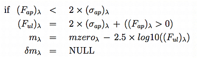
When the WPRO or WAPP flux measurement has a signal-to-noise ratio less than 2, the respective WPRO or WAPP calibrated magnitude in the Working Database is replaced with the 2-σ brightness upper limit in magnitude units. In these cases, the magnitude uncertainty values are set to NULL.
The magnitude upper limit is computed by replacing the integrated flux measurement with the flux measurement plus two times the measurement uncertainty, as shown below. If the integrated flux measurement is negative, then the flux is replaced with two times the flux uncertainty.
 |
(Eq. 36) |
| (Eq. 37) | |
| (Eq. 38) | |
| (Eq. 39) |
where mzeroλ is the instrumental zero point magnitude (IV.4.h), mλ is the reported upper limit in mag units, and its uncertainty δmλ is set to NULL.
Sources that are in close proximity (xscprox <= 2 arcsec) to 2MASS XSC sources are assumed to be associated (i.e., the same source), and special is triggered for the source. The aperture is based on the elliptical shape that the 2MASS XSC reports. Due to the larger WISE beam, however, the aperture is adjusted (scaled) accordingly. Fig. 12 illustrates the difference in beam between 2MASS, IRAC and WISE, and the plots (Fig. 13-14) that follow show the quantitative difference which WAPPco uses to adjust the elliptical aperture for a particular case (XSC size and inclination). For a full suite of sizes and shapes, a lookup table is created to adjust the WISE aperture in accordance with the 2MASS XSC aperture shape.
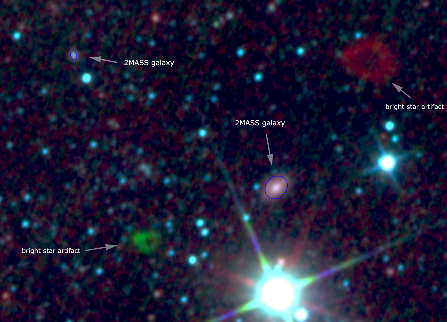 |
| Figure 11 - WISE W1+W2+W3 composite image showing the elliptical aperture (blue) used to extract the flux from 2MASS galaxies in the field. |
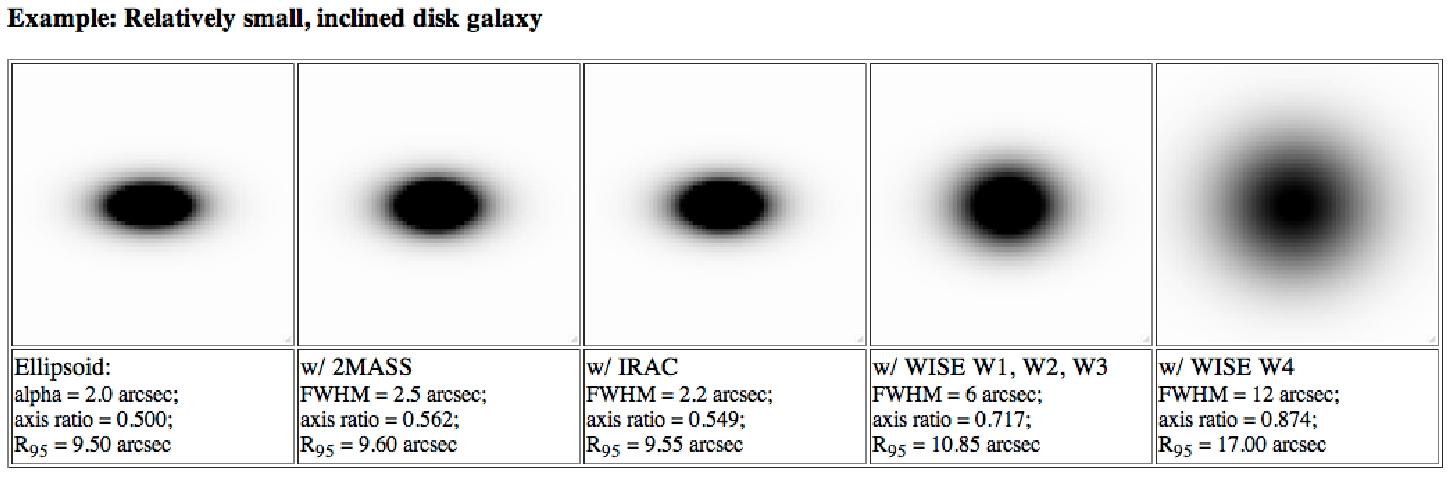 |
| Figure 12 - Comparing 2MASS, IRAC and WISE beam-convolution of an ellipsoid model. the ellipsoid is defined as: f = f0 * exp(-r / alpha), where r is the radius based on the ellipse with axis ratio and position angle parameters; R95 represents the semi-major axis at which 95% of the total flux is captured. |
 |
 |
| Figure 13 - Semi-major axis of the disk galaxy compared to the actual radius due to the beam resolution. | Figure 14 - Axis ratio departure from 0.5 due to the beam resolution. |
 |
| Figure 15 |
 |
| Figure 16 |
 |
| Figure 17 |
 |
| Figure 18 |
 |
| Figure 19 |
 |
| Figure 20 |
Photometric measurements of large (well resolved) sources made on the coadded Atlas Images require a correction to the integrated flux in order to conform with the WISE absolute photometric calibration which is based on profile-fitting of point sources.
Profile-fiting photometry captures most of the flux of a source, but because of the finite size of the single-exposure PSFs used during second-pass data processing, a few percent of the source flux was not captured. This does not affect point source photometry because all sources are measured exactly the same way, including the photometric calibration stars. However, measurements that attempt to capture the total flux of sources on the Atlas Images will systematically overestimate the the total brightness because the standard stars are measured with finite sized PSFs. To compensate for this bias, a small "aperture" correction must be applied as follows:
| W1 | W2 | W3 | W4 |
| [mag] | [mag] | [mag] | [mag] |
| -0.034 | -0.041 | +0.03 | -0.029 |
The value of the aperture corrections given above are derived from the characteristic curve-of-growth of the PSF on the coadded Atlas Images, as described in IV.4.c.viii. Because the PSF on each Atlas Image is unique, these corrections are approximate and may vary slightly between images.
There is no single PSF or set of PSFs that characterize point sources on the WISE Atlas Images.
WISE Atlas Images are constructed by coadding many single-exposure images (IV.4.f). Because the number and relative orientation of single-exposures differ significantly between Atlas Tiles, and because the single-exposure PSFs vary with focal plane location (IV.4.c.iii), the PSF will be different for every Atlas Image and will vary with position on any given Atlas Image.
WISE Multiframe pipeline photometry is done by fitting PSFs simultaneously on all single-exposures contributing to the Atlas Image. The PSF appropriate for the respective focal plane positions on each single-exposure images are used.
The most accurate method of doing any analysis that requires a PSF for an Atlas Image is to measure the PSF empirically from the image that is being measured.
Nonetheless, it is useful to examine the characteristic PSF from an ensemble of Atlas Images to derive certain corrections for measurements made on the images.
Built from the deep WISE surveys of the Ecliptic Poles (Jarrett et al. 2011) and of the ELAIS N1 region, the Point Spread Function (PSF) per WISE band is presented in this document. These PSFs correspond to co-added "mosaics" constructed from many hundreds of frames (per band) collected over the lifespan of the cryo-genic survey. The spacecraft orientation fully rotated over this period of time, circularizing and averaging out focal plane distortions and other asymetries in the spacecraft and detector optics. Hence, the Ecliptic Pole PSFs represent the "ideal" set for WISE coadded images.
We present the PSFs (fits images), their associated uncertainty (fits images) and the curves of growth per band (tabular data). We note the "aperture" correction that is required to adjusted total flux measurements from co-added mosaics to the photometric calibration adopted for WISE.
Note: The co-added "mosaic" PSFs should not be confused with the single-exposure frame PSFs that were used to extract photometry during the pipeline processing. Rather, the coadd PSFs are relevant to any direct measurements using the co-added mosaic images.
For comparison, we show the aperture correction used to adjust the standard aperture photometry (WAPPco) to match the profile-fitting photometry (WPRO). In principle, this aperture correction should transform the small aperture measurement to a total measurement; however, since WPRO does not extract the total flux, there is a small difference between this aperture correction and the curve-of-growth correction. This small difference represents a correction that is needed to bring the coadd "total" measurements onto the WISE calibration system.
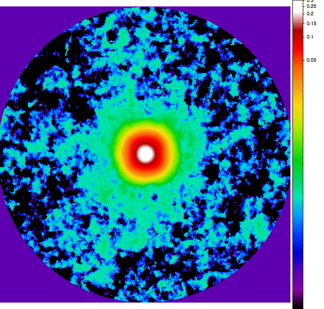
W1 Point Spread Function (PSF) constructed from co-added "mosaics" of the deep Ecliptic Pole observations. The data is encapsulated in the FITS image and its associated uncertainty image. |
W2 Point Spread Function (PSF) constructed from co-added "mosaics" of the deep Ecliptic Pole observations. The data is encapsulated in the FITS image and its associated uncertainty image. |

W3 Point Spread Function (PSF) constructed from co-added "mosaics" of the deep Ecliptic Pole observations. The data is encapsulated in the FITS image and its associated uncertainty image. |
W4 Point Spread Function (PSF) constructed from co-added "mosaics" of the deep Ecliptic Pole observations. The data is encapsulated in the FITS image and its associated uncertainty image. |
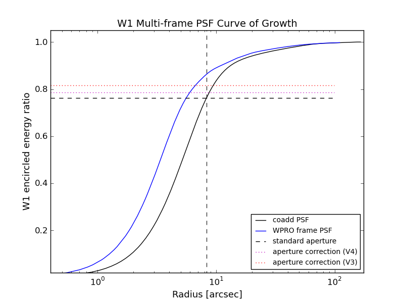
W1 PSF curve of growth. The encapsulated energy represents the correction needed to transform the circular aperture photometry (radius R) to a total flux: measured flux / encapsulated energy. The dashed line demarks the "standard" aperture (8.25" radius) measurement used in the WISE pipeline processing; the grey dotted line denotes the correction needed to transform the standard flux to a total flux. For comparison, we show the aperture correction (red dotted line) used to adjust the standard aperture photometry (WAPPco) to match the profile-fitting photometry (WPRO). |
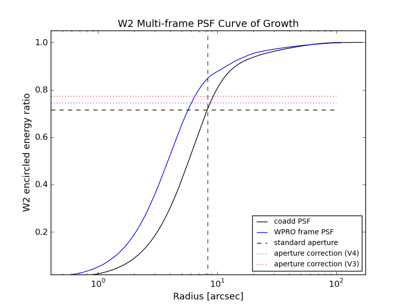
W2 PSF curve of growth. The encapsulated energy represents the correction needed to transform the circular aperture photometry (radius R) to a total flux: measured flux / encapsulated energy. The dashed line demarks the "standard" aperture (8.25" radius) measurement used in the WISE pipeline processing; the grey dotted line denotes the correction needed to transform the standard flux to a total flux. For comparison, we show the aperture correction (red dotted line) used to adjust the standard aperture photometry (WAPPco) to match the profile-fitting photometry (WPRO). |
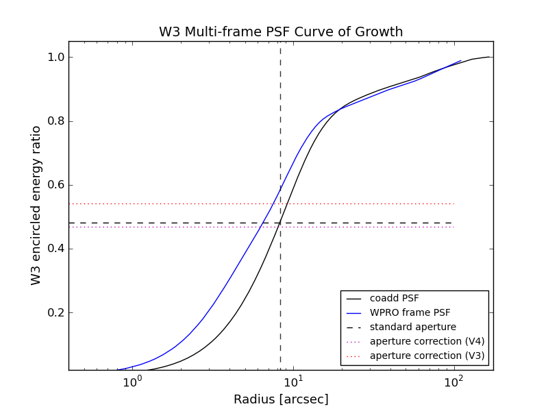
W3 PSF curve of growth. The encapsulated energy represents the correction needed to transform the circular aperture photometry (radius R) to a total flux: measured flux / encapsulated energy. The dashed line demarks the "standard" aperture (8.25" radius) measurement used in the WISE pipeline processing; the grey dotted line denotes the correction needed to transform the standard flux to a total flux. For comparison, we show the aperture correction (red dotted line) used to adjust the standard aperture photometry (WAPPco) to match the profile-fitting photometry (WPRO). |
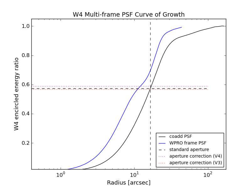
W4 PSF curve of growth. The encapsulated energy represents the correction needed to transform the circular aperture photometry (radius R) to a total flux: measured flux / encapsulated energy. The dashed line demarks the "standard" aperture (16.5" radius) measurement used in the WISE pipeline processing; the grey dotted line denotes the correction needed to transform the standard flux to a total flux. For comparison, we show the aperture correction (red dotted line) used to adjust the standard aperture photometry (WAPPco) to match the profile-fitting photometry (WPRO). |
| Figures 21a and 21b – W1 | Figures 22a and 22b – W2 | Figures 23a and 23b – W3 | Figures 24a and 24b – W4 |
Last update: 2018 July 9