


First, we strongly advise you search the WISE Source Catalog for objects of interest, and use photometric measurements therein if available. Otherwise, for objects that didn't satisfy the catalog selection criteria, or for extended sources/emission where PSF-fit photometry is unreliable (see section IV.4.c.iii), we outline below a recommended method for performing aperture photometry with uncertainty estimation using the Atlas Image products. These are primarily the intensity and uncertainty maps. Particular attention is given to uncertainty estimation in the presence of correlated noise - a feature of the Atlas Images. The uncertainty estimation methodology can be applied to (by rescaling) the outputs from most photometry packages, including those that perform PSF-fit photometry. Here we summarize the main equations.
In general, the flux of a source (in image-pixel units of DN) within an aperture containing NA pixels can be computed from:
 |
(Eq. 1) |
where Ftot is the sum of all pixel fluxes in the source (measurement) aperture and B is a robust measure of the local background level per pixel (robust against outliers and other contaminating sources, e.g., a mode, trimmed mean or trimmed median), usually estimated from an annulus around the source aperture. fapcor is the aperture correction factor, whose equivalent in magnitudes is: mapcor = -2.5log10(fapcor).
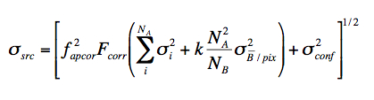
The corresponding 1-σ uncertainty in Fsrc (Eq. 1), also in DN, is given by:
 |
(Eq. 2) |
where
NA = number of pixels in source aperture.
NB = number of pixels in source annulus.
σi = flux uncertainty for pixel i from uncertainty map, rescaled if necessary to ensure consistency with local RMS fluctuations at fixed depth-of-coverage as described in section II.3.e.i.
Fcorr = correlated noise correction factor for flux variance (see section II.3.f.i below).
B = robust background estimate per pixel in annulus (e.g., trimmed mean or trimmed median).
k = 1 if B = mean background/pixel, or mean-related measure; k = π/2 if B = median background/pixel, or median-related measure.
σ2B/pix = Variance in sky-background annulus. Can estimate from the squared median or trimmed mean of σi values over pixels i in annulus off the uncertainty map. In regions with low confusion and a spatially uniform background, can also compute from the square of some robust estimator of the RMS fluctuation, e.g., using inter-percentile ranges: ≈ [0.5(P84% - P16%)]2 ≈ (P50% - P16%)2, or the Median Absolute Deviation from the median (MAD): [1.4826median{|pi - median{pi}|}]2.
σ2conf = Confusion noise-variance
on scale represented by measurement aperture (see section
II.3.f.ii below).
We have assumed the uncertainty in the aperture correction (fapcor) is negligible since usually it can be determined to good accuracy. The aperture corrections for a limited set of aperture sizes used on Atlas Images when constructing the WISE Source Catalog can be found in section IV.4.c.iv.2. Note also the additional (small) corrections described in section IV.4.c.vii (even when using very large apertures) in order to obtain the correct absolute calibration when using the conversion factors in Table 1.
To convert the raw Fsrc and σsrc DN measurements from Eqns (1) and (2) respectively to calibrated magnitudes (relative to WISE standards), the following equations should then be used:
 |
(Eq. 3) |
The "1.179" factor comes from (2.5/loge10)2 and MAGZP is the magnitude zero-point with corresponding uncertainty σMAGZP. These are represented by FITS keywords MAGZP and MAGZPUNC respectively in the headers of all Atlas Images (see also Table 1). These values are the same for all Atlas Images of a given band since all the single exposures were throughput (gain)-matched to a common photometric zero-point prior to coaddition.
The single exposure photometric zero points (section IV.4.h.iii) were observed to be relatively stable with a uniform scatter throughout the cryogenic phase of the mission (encompassing the all-sky release described here). The MAGZPUNC values in Table 1 reflect the absolute uncertainty in the mean MAGZP values derived from a Spitzer-MSX-WISE cross-calibration prior to commencement of all-sky processing (for details, see Jarrett et al. 2011). The accuracy of the MAGZP values may improve in future.
As a side note, photometric uncertainties reported in the WISE Source Catalog do not fold in the uncertainty in MAGZP as shown in Eq. (3). The components contributing to σsrc for the catalog uncertainties are similar to those in Eq. (2), but include a PSF-estimation error term for measurements based on profile-fit photometry (for details, see section IV.4.c.iii).
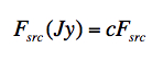
Given some magnitude, MAG, the absolute flux density (e.g., Jy) can be computed using f = f010-0.4MAG, where f0 is the absolute flux for MAG = 0 for your band of interest. Alternatively, you could simply apply a DN-to-Jy conversion factor to the outputs from Eqs (1) and (2). More precisely, if c is the DN-to-Jy conversion factor (listed in Table 1), then your raw aperture photometry estimates (Fsrc and σsrc in DN from Eqs 1 and 2) can be converted to units of Jy using:
 |
(Eq. 4) |
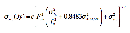 |
(Eq. 5) |
where 0.8483 ≈ (0.4loge10)2 and all other calibration constants and their uncertainties are listed in Table 1.
| Band | MAGZP [mag] |
MAGZPUNC (= σMAGZP) [mag] |
f0[1] [Jy] |
σf0[1] [Jy] |
DN-to-Jy conv. (= c)[2] [Jy/DN] |
|---|---|---|---|---|---|
| 1 | 20.5 | 0.006 | 306.682 | 4.600 | 1.9350E-06 |
| 2 | 19.5 | 0.007 | 170.663 | 2.600 | 2.7048E-06 |
| 3 | 18.0 | 0.015 | 29.0448 | 0.436 | 1.8326e-06 |
| 4 | 13.0 | 0.012 | 8.2839 | 0.124 | 5.2269E-05 |
Correlated noise usually occurs in re-sampled and interpolated images with the degree of correlation depending on the extent of the interpolation kernel and ratio of input-to-output pixel size (for details, see section IV.4.f.vii). The smoothing (interpolation) kernel used to create a WISE Atlas Image has moved noise-power from high to low spatial frequencies and therefore needs to be recaptured to properly quantify the uncertainty in the flux summed over a region. Ignorance of correlated-noise will lead to an underestimate of the final photometric uncertainty, sometimes by an appreciable amount. This is the purpose of the correlated-noise correction factor Fcorr in Eq. (2).
Since the Atlas Images were created using the detector PRF as the interpolation kernel (section IV.4.f.vii), it can be shown that Fcorr ≈ Np(sin/sout)2 where Np is the effective number of noise-pixels characterizing the PRF, in terms of the number of native detector pixels, and sin/sout is the ratio of input (detector) pixel scale to output (Atlas Image) pixel scale. This ratio is ≈ 2 for W1, W2, W3, and ≈ 4 for W4. This is a good approximation for apertures containing NA >~ 50Np pixels. For significantly smaller apertures, Fcorr is smaller and can be approximated to ~10% accuracy using Figures 1-4 for a given aperture radius measured in co-add (Atlas Image) pixels. These figures apply only to the WISE-band PRFs and output co-add pixel size (1.375 arcsec), and were derived using Monte-Carlo simulations of co-added frames with input Gaussian noise.
 |
 |
| Figure 1 - Fcorr vs aperture radius for W1 [click to enlarge]. Download digital version. | Figure 2 - Fcorr vs aperture radius for W2 [click to enlarge]. Download digital version. |
 |
 |
| Figure 3 - Fcorr vs aperture radius for W3 [click to enlarge]. Download digital version. | Figure 4 - Fcorr vs aperture radius for W4 [click to enlarge]. Download digital version. |
The confusion-noise term in Eq. (2), σconf, represents the contribution to the image-noise from the superposition of faint and unresolved sources on scales equivalent to the measurement aperture. Confusion noise becomes important in regions of high source density, typically when the surface density down to the instrumental and background-Poisson noise limit for the image at hand exceeds ~1/30 sources beam-1 (Condon, 1974), although this drops to ~1/50 sources beam-1 when the number-flux relation is Euclidean or steeper (e.g., Hogg, 2001). Taking a "beam" to be the solid angle spanned the FWHM of the effective PSF for WISE Atlas Images (~8.5 arcsec in bands W1,W2,W3, and ~17 arcsec in W4), the 1/30 beam-1 criterion translates to ~2 sources arcmin-2 for W1,W2,W3, and ~0.5 sources arcmin-2 for W4.
The confusion noise component is measured as an excess above any correlated instrumental and background-Poisson pixel-noise on these scales. It can be derived empirically from the background image RMS fluctuation on measurement-aperture scales if one has prior knowledge the instrumental and background-Poisson components in their region at the given depth-of-coverage (i.e., as provided by the uncertainty maps). For example, if σapbck is the background RMS fluctuation on measurement-aperture scales, we have
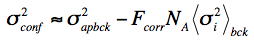 |
(Eq. 6) |
where <σ2i>bck is a robust estimate (e.g., median or mode) of the noise-variance per pixel over the background region of interest from the uncertainty map. Note: the noise-variance is the square of pixel values in this map. NA is the number of pixels in your measurement aperture. The estimation of σaptot involves throwing many apertures of size NA at random, summing the pixel flux in each (to yield a flux of FAj for aperture j), and then retaining those apertures that (i) don't significantly overlap with another (so spatial correlations are minimized), and (ii) fall within regions with a relatively uniform, source-free background. σaptot is then the RMS over all remaining FAj values. The difficulty here is having enough random samples (apertures) that are not significantly contaminated and cover a spatially-uniform background.
Alternatively, the confusion noise can be predicted using star or galaxy count models for your field and knowledge of the WISE beam or measurement aperture (e.g., Väisänen et al. 2001). Note that the Atlas Image derived confusion noise and its comparison to predictions from star/galaxy count models for WISE has not yet been studied in detail.
Last update: 2012 July 27