


All magnitudes listed in the WISE Source Catalog and Single-Exposure Source Database have been photometrically calibrated using observations of a network of standard stars that are located near the ecliptic polar caps, as described in IV.4.h.ii. For WISE Atlas and Single-exposure Images, photometric zero points that allow direct conversion of pixel intensity values to calibrated magnitudes, are derived for calibrators throughout the WISE mission. The photometric zero point values are provided in the MAGZP keyword values in the FITS image headers.
This section on Photometric Calibration describes in more detail the process by which instrumental source magnitudes were converted to calibrated magnitudes, and how the photometric zero point levels were derived for WISE. A brief introduction to the WISE photometric system is given below. Additional information can be found in Wright et al. (2010 AJ, 140, 1868) and Jarrett et al. (2011 ApJ, 735, 112).
All reported magnitudes are in the Vega System. Formulae for converting WISE Vega magnitudes to flux density units (in Janskys) and AB magnitudes are given below along with two practical examples.
The source flux density, in Jansky [Jy] units, is computed from the calibrated WISE magnitudes, mvega using:
 | (Eq. 1) |
where  is the zero magnitude flux density
corresponding to the
constant that gives the same
response as that of Alpha Lyrae (Vega).
For most sources,
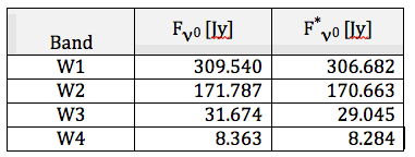
the zero magnitude flux density, derived using a constant power-law spectra, is appropriate and may be used to convert WISE magnitudes to flux density [Jy] units. Table 1 lists the zero magnitude flux density (column 2)
for each WISE band.
is the zero magnitude flux density
corresponding to the
constant that gives the same
response as that of Alpha Lyrae (Vega).
For most sources,
the zero magnitude flux density, derived using a constant power-law spectra, is appropriate and may be used to convert WISE magnitudes to flux density [Jy] units. Table 1 lists the zero magnitude flux density (column 2)
for each WISE band.
For sources with steeply rising MIR spectra or with spectra that deviate significantly from Fν=constant, including cool asteroids and dusty star-forming galaxies, a color correction is required, especially for W3 due to its wide bandpass. With a given flux correction, fc, the flux density conversion is given by:
 | (Eq. 2) |
 , listed in Table 1 (column 3)
and the flux correction, fc, listed in Table 2 for
, listed in Table 1 (column 3)
and the flux correction, fc, listed in Table 2 for
 ,
where the index α ranges from: -3, -2, -1, 0, 1, 2, 3, and 4, and for blackbody spectra, Bν(T) for a variety of temperatures,
and for stars of two main-sequence spectral types (K2V and G2V).
,
where the index α ranges from: -3, -2, -1, 0, 1, 2, 3, and 4, and for blackbody spectra, Bν(T) for a variety of temperatures,
and for stars of two main-sequence spectral types (K2V and G2V).
 where  ; in the third column,
, and is used for
color corrections such that ; in the third column,
, and is used for
color corrections such that  , where fc is
the flux correction given in Table 2. , where fc is
the flux correction given in Table 2.
|
|
Because of uncertainty in the calibration of the W4 Relative Spectral Response
(RSR), sources that have a steeply rising mid-IR spectrum,
where α >= 1,
require approximately an 8 to 10% correction to the W4 flux, as follows:
 | (Eq. 3) |
Additional details are given in Discrepancy between blue and red source measurements.
Monochromatic AB magnitudes are defined by
 (see e.g., Tokunaga
& Vaca 2005).
Hence, conversion from the WISE Vega-system magnitudes to flux density using
(see e.g., Tokunaga
& Vaca 2005).
Hence, conversion from the WISE Vega-system magnitudes to flux density using
![]() (column 2 of Table 1)
and to AB magnitudes follows:
(column 2 of Table 1)
and to AB magnitudes follows:
 | (Eq. 4) |
| Band | magnitude offset (Δm) |
|---|---|
| W1 | 2.699 |
| W2 | 3.339 |
| W3 | 5.174 |
| W4 | 6.620 |
Case 1 (blue source) -- WISE J091538.49+095230
WISE J091538.49+095230 is a QSO at z= 0.62 (SDSS J091538.48+095230.0),
a relatively "blue" extragalactic object that is well detected in the
first three WISE bands and detected, but quite faint (SNR ~ 4) in W4.
The profile-fit magnitudes
(w?mpro) in the All-Sky Release
Catalog for this sources are listed in column 2 of Table 4.
The colors of this source are: [W1-W2] = 1.16 mag and [W2-W3] = 2.85 mag.
Looking at the spectral colors in Table 2, the source appears to have spectral
slope that is somewhat flat, an index between "0" and "1" for
Finally, as noted above, most stars and galaxies (with α < 1) do not
require a color correction. Simply using the constant power-law
conversion,
Case 2 (red source) -- WISE J145606.01+193839.6
This strikingly red WISE source is associated with the IRAS source
IRAS F14537+1950 (z = 0.64), a starbursting hyperluminous infrared galaxy.
The WISE All-Sky Release Catalog photometry for this source is given in
column 2 of Table 6, below.
The colors of this source are: [W1-W2] = 0.48 mag and [W2-W3] = 4.03 mag.
Looking at the spectral colors in Table 2, the source appears to have an index
between "2" and "3" for
Note that adopting the flat-spectrum constant WISE is calibrated on the same absolute basis as that established for the
Spitzer Space Telescope. Networks of calibration stars support Spitzer
observations with IRAC, MIPS and IRS, further providing cross-calibration
between all three instruments. IRAC's primary suite of standard calibration
stars lies in the north ecliptic pole continuous viewing zone
(Reach et al. 2005
PASP, 117, 978). Their stellar energy distributions were constructed by
Cohen et al. (2003, AJ, 125, 2645) to tie directly
to the absolute mid-infrared calibrations by Midcourse Space Experiment MSX
(Price et al. 2004,
SSRv 113, 409). Japan's AKARI mission uses
the identical techniques and is tied to Spitzer by having absolute calibrators
in common, drawn from the same networks
(Ishihara et al.
2006, PASP, 118, 324). It was natural that WISE adopted the same
approach to absolute and relative calibration
so that data from all of these infrared missions can be simply co-analyzed.
The WISE team, in collaboration with the Spitzer Science Center, carried out
a survey of the north and source ecliptic poles (NEP and SEP), the WISE
"continuous viewing zones" (CVZs), using the
full complement of Spitzer instrumentation: IRAC and MIPS
broad-band mapping of a 47x47 arcmin (0.6 deg2) region for each CVZ,
and IRS spectroscopy of either previously identified calibrator stars or newly
developed standard calibrators.
The imaging and spectroscopic observations include the galaxy NGC 6552, which
is used to cross-calibrate the long-wavelength band of WISE with the
Spitzer IRS-LL and MIPS 24 micron channel.
The polar surveys were used to (i) provide consistent calibrators in both of
the WISE CVZs, (ii) develop new calibrators near the south ecliptic pole
where few existed previously , (iii) establish the
photospheric character of all candidate calibrators, (iv) assess the long-term
stability for secondary standards, (v) identify objects that would saturate the
WISE arrays, (vi) identify galaxies that are resolved by IRAC, and measure
their properties using methods appropriate to extended sources, and
(vii) study the extragalactic population.
The observations, results and analysis are presented in
Jarrett et al.
(2011).
Because of the scarcity of W4 calibrators near the ecliptic poles, a set of
W4 calibrators located further from the poles are selected to supplement the
initial set of W4 WISE calibrators. The complete set of WISE photometric calibrators is listed in Tables 7a-7d.
The instrumental source brightness measurements made by the pipeline photometry
module (IV.4.c) are calibrated by adding
an instrumental zero point magnitude. The calibrated magnitudes
given in the WISE All-Sky Release Source Catalog and Single-exposure Source
Database magnitudes are given by:
where
The instrumental zero point magnitudes are band-dependent,
and are different for the photometry in the All-Sky Release
Catalog/Reject Table and Single-exposure Source Database.
The zero point derivation is described
in IV.4.h.iv.
The instrumental zero point magnitudes for photometry on the Single-exposure
images were derived using the measurements of the
calibration sources made during each scan.
The zero point magnitudes, M0,inst, were
computed for each band, b, and are equal to the average difference
between
the prior, "true" magnitude of each calibrator and the instrumental
magnitude measured by the Scan/frame Pipeline.
where Mp,b is the prior, "true" magnitude of the calibrator,
and Mm,b is the measured, instrumental
magnitude in band, b. The instrumental zero points used for the
Single-exposure Source Database for the full cryogenic survey phase are
listed in Table 8.
The RMS values listed are the root variance of the differences between the
true and measured magnitudes for all calibration source measurements.
The standard deviations of the mean instrumental zero points are <<1%
for all bands because thousands of measurements are used to evaluate them.
The Single-exposure database instrumental zero point magnitudes
are also carried in the MAGZP values in the Single-exposure
FITS headers and
w?zero values in the
Frame Metadata Table.
Initial estimates of the Single-exposure instrumental zero point values
were made early in the WISE survey and were used to calibrate photometry
during first-pass processing.
The zero points were refined prior to
second-pass processing
and were based on analysis of all measurements of the calibration
sources over the full cryogenic survey phase.
The instrumental zero point magnitudes used to calibrate
source measurements in the Multiframe Pipeline
for the All-Sky Release Source Catalog and Reject Table are selected
values that are similar but not identical to the Single-exposure
instrumental zero points.
Pixel values in each of the Single-exposure images contributing to
an Atlas Image were scaled to a common gain in the
throughput matching step of the
Atlas Image Generation module, using factors computed from the
instrumental zero points of the individual exposures and the pre-defined
Atlas Image zero point. This scaling step was designed to accomodate
possible changes in the system throughput throughout the survey.
No measurable throughput changes were seen during the full cryogenic survey
phase, but significant changes were measured during the
3-Band Cryo and Post-Cryo
phases. The Catalog and Reject Table instrumental zero point
magnitudes listed in Table 8 are also carried in the
MAGZP values in the Atlas Image FITS headers and
w?magzp values in the Atlas Image
Metadata Table.
In Figures 3a through 3d are shown the differences between true and
measured Single-exposure magnitudes that have been
calibrated
using the instrumental zero points in Table 8, for all calibrators, plotted
as a function of time. For W4 in figure 3d, the blue and red points
represent the residuals for stellar (blue) calibrators
and the Seyfert galacy NGC6552 (red) calibrator, respectively.
The discrepancy between the blue and red source measurements is
discussed in IV.3.g.vii.
These residual time histories illustrate that the WISE system
photometric throughput was extremely stable over the period of the
full cryogenic survey.
The average residuals between true and measured magnitudes is 0.008, -0.001,
-0.001 and 0.028 mag in the four bands, respectively.
The WISE photometric stability is even better than represented by
Figures 3a-3d. Some of the apparent scatter in the
time histories of the photometric residuals comes from uncertainty in the
knowledge of the "true" brightness of the calibration sources. Figures
4a-4c show the time history of the W1-W3 zero point residuals, as in
Figures 3a-3c, but in each of these plots residuals from a single calibrator
are shown in green. The scatter in the single source distributions is
noticeably smaller than for the ensemble, and the corresponding
RMS values are commensurate: 0.023, 0.024 and 0.025 mag in
W1, W2 and W3, respectively. Only one of the W4 calibration sources,
NGC6552, is near an ecliptic pole and was therefore monitored
continuously during the survey. The blue calibrators are all at lower
ecliptic latitudes, and thus different calibrators are observed at
different times. This combined with inherent uncertainties in their
true 22μm fluxes produces the apparent
large temporal variation in the residuals seen in Figure 3d.
The WISE relative system response curves (RSRs) were created from the end-to-end
lab measurements by modifying the prediction and design values at each wavelength
by fitting a line in log-log space and using this to replace any originally negative values.
Following the prescription of Bessell (2000), we convert the QE-based
Wright et al. (2010)
RSRs (Fig. 5) from electrons per photon to photon-counting response curves by multiplying by λ
and renormalizing each curve to a peak of unity; see Fig. 5b.
Both W1 and W2 passbands have close correspondence with those of IRAC-1 and IRAC-2,
although the W1 passband is slightly `blue' compared to IRAC-1 and W2 is slightly `red' compared to IRAC-2.
The reddest channel of WISE, W4 at 22 µm, compares well with MIPS-24, although it is
slightly bluer in response. Compared to Spitzer imaging, the only unique band of WISE
is that of W3 (12 µm) which has only small overlap with that of IRAC-4 (8 µm),
but is comparable to the IRAS 12 µm channel. One consequence of this band-to-band
difference is demonstrated in Fig. 4b, the spectrum of ultra-luminous infrared
galaxy Arp 220 has strong polycyclic aromatic hydrocarbon (PAH) emission bands,
notably at 11.3 µm compared to the bands at 6.2 and 7.7 µm.
WISE W3 compared to IRAC-4 will be more sensitive to both PAH emission
and amorphous silicate absorption (10 µm) in nearby star-forming galaxies.
Moreover, because W3 is a longer wavelength channel than IRAC-4,
it is more sensitive to higher redshift galaxies in which strong
near-IR continuum and mid-IR emission features redshift into the band.
The QE-based RSRs in ASCII table format are available for
W1,
W2,
W3, and
W4,
which includes wavelength in microns, the response, and the uncertainty in the response in parts per thousand
(from Wright et al. 2010).
The response per unit energy RSRs in ASCII table format are available for
W1,
W2,
W3, and
W4,
which include wavelength in microns, the response, and the uncertainty in
the response in parts per thousand (from
Jarrett et al.
2011).
Adopting a stellar photospheric spectrum, specifically that for an "ideal" Vega in which
the effective temperature is uniform across the stellar surface (described in Cohen et al. 1992),
the system, or isophotal wavelengths, λ(iso), are found to be
3.35, 4.60, 11.56, and 22.08 µm (see also Wright et al. 2010).
The isophotal flux Fλ(iso) was derived by integrating the modified Vega spectrum across the WISE
RSRs. For the frequency equivalent integral, Fν(iso), we applied the method described in Cohen et al. (1999)
and Tokunaga & Vacca (2005), recasting each WISE RSR in frequency terms and integrating the
stellar spectrum over the RSR to derive the in-band flux. The resultant isophotal quantities
and other WISE system attributes are given in Table 8 for both wavelength-based and frequency-based RSRs.
Note that Wright et al. (2010) use a different treatment to calculate the Fν(iso)
values that is based on the direct conversion of λ(iso) to Fν using the formulation
Fν(iso) equals (λ2(iso)/c)Fλ(iso);
this method is strictly an approximation used for narrow-band filters and is
typically unsuitable for wide passbands (Cohen et al. 1999, their Sec. 3.3; and the
standard method is restated by Tokunaga & Vacca 2005).
The approximation is in fact adequate for W1, W2 and W4.
Wright et al. (2010)
provide a set of flux corrections, fc, that properly transform from Fν*(iso) to `in-band'
Fν(iso): Absolute measurements of stars and comparisons of stellar irradiances with those of emissive
reference spheres were made by MSX. This `ideal' Vega spectrum was absolutely validated by
photometry on the MSX and provided the basis for defining the zero magnitude for Infrared
Space Observatory (ISO), MSX, Spitzer, and AKARI infrared space telescopes. This validated
zero magnitude system is traceable to measurements using K (primary) and M giant (secondary)
calibrators and has an absolute precision of ±1.10%. This basis now serves the same purpose
for the four WISE bands, ensuring that their photometric calibrations have been computed
in the same manner as for these previous missions. The in-band fluxes of the Vega spectrum were adopted to define zero magnitude for WISE bands
W1, W2, and W3. Data for W4 incorporate the 2.7% upward offset from the Vega basis model
that was established absolutely by MSX at 21.3 µm (Price et al. 2004: Table 4, Column 7,
and Table 9, Column 2), and applied by Cohen (2009) in the validation of the diffuse
calibration of Spitzer MIPS-24 by comparison with the MSX 21.3 µm band. This Vega basis has
an overall systematic uncertainty of ~1.45%.
Photometric performance is gauged using the individual and time history
measurements of the WISE calibrators. The RMS residuals in the zero point
offset for each WISE band (Table 8) provide a measure
of the accuracy of the calibration solution, while the time history provides
a metric for the photometric stability over the lifetime of the cryogenic
mission (Figure 3).
Figure 6 shows the time history of the difference between the
predicted (true) and measured magnitudes for the
ensemble of calibration stars, average in coarse time bins.
In Figure 7 are shown the mean and standard deviation of the
flux residuals for each calibration source, plotted as a function of
the source brightness.
Time variability in the instrumental zero point magnitude is ruled out with
individual (repeated) measurements over the lifetime of the mission;
repeated observations of the individual calibrators reveal an RMS scatter,
typically better than 1% (Figure 6).
In contrast, the ensemble plotted in Figure 7 has a much larger scatter
than the trending in the zero point.
For both W1 and W2, the inverse variance-weighted mean is 0.007 +- 0.025 mag,
for W3 it is 0.017 &plusm; 0.045 mag, and
for W4, it is -0.021 &plusm; 0.057 mag.
The ensemble results suggest that the WISE absolute calibration, tied to
that of Spitzer, has an RMS scatter in the standard calibration stars at
the 2.4, 2.8, 4.5 & 5.7% levels for W1, W2, W3 and W4, respectively.
The observed scatter in Figure 7 arises chiefly from the uncertainty in the
predicted WISE flux values for the calibration sources, reflecting the
inherent errors associated with model fitting to the broad-band SED
measurements, as well as the uncertainty in the WISE RSRs. These errors
are much larger then the expectation at the
longer mid-IR wavelengths, notably in the W4 window -- the red calibrator
NGC 6552 has a W4 residual of ~6%, a difference that appears to be systematic
for very red sources as measured using Spitzer-IRS spectra from ultra-luminous
infrared galaxies
(see Wright et al. 2010).
Photometric calibration is based on measurements of bright stars, A-K
dwarfs and K/M giants, which are relatively blue in color in comparison
to star-forming galaxies, for example. As shown in
Figures 3d above, the Sy-2 galaxy NGC 6552 appears to
have a significantly different zero point offset compared to the bluer stellar
calibrators. This difference has been observed
in other red extragalactic objects, notably ultra-luminous infrared galaxys
(ULIRGs).
Wright et al.
(2010) describe the blue vs. red calibration discrepancy as follows:
Brown
et al. (2014) find that the residual between W4 Source Catalog photometry
and photometry synthesized using spectral energy distributions for
galaxies can be approximated by the functional form:
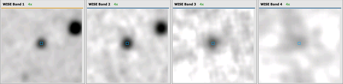
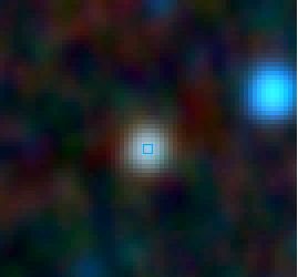
Figure 1a - WISE W1, W2, W3 and W4 Atlas Images of source
J091538.49+095230. The field of view is 90 arcsec.
Figure 1b - 3-color composite image: blue = W1, green = W2, red = W3.
band
w?mpro (unc)
Fν(corr) (unc)
mag
mJy
W1 14.474 (0.035) 0.50 (0.02)
W2 13.318 (0.037) 0.81 (0.03)
W3 10.465 (0.082) 2.02 (0.15)
W4 8.059 (0.245) 4.99 (1.13)
.
For a slope of "1", the corresponding flux corrections are: 0.992, 0.994,
0.937, 0.993, applied with .
The corrected, monochromatic (λiso) flux densities after
application of the flux corrections are listed in column 3 of Table 4
![]() (column 2 of
Table 1) provides a reasonable conversion to flux density.
The monochromatic flux densities using the constant power-law conversion
are listed in Table 5, and are nearly identical to the color-corrected
versions shown in Table 4.
(column 2 of
Table 1) provides a reasonable conversion to flux density.
The monochromatic flux densities using the constant power-law conversion
are listed in Table 5, and are nearly identical to the color-corrected
versions shown in Table 4.
band
w?mpro (unc)
Fν(corr) (unc)
mag
mJy
W1 14.474 (0.035) 0.50 (0.02)
W2 13.318 (0.037) 0.81 (0.03)
W3 10.465 (0.082) 2.06 (0.15)
W4 8.059 (0.245) 5.00 (1.13)
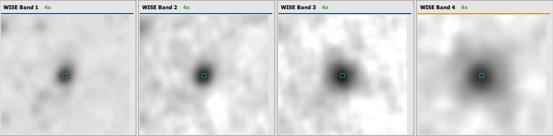
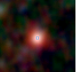
Figure 2a - WISE W1, W2, W3 and W4 Atlas Images of source
J145606.01+193839.6. The field of view is 90 arcsec.
Figure 2b - 3-color composite image: blue = W1, green = W2, red = W3.
band
w?mpro (unc)
Fν(corr) (unc)
mag
mJy
W1 14.492 (0.029) 0.49 (0.01)
W2 14.012 (0.037) 0.42 (0.01)
W3 9.985 (0.038) 2.94 (0.10)
W4 6.656 (0.056) 16.58 (0.86)
.
The corresponding flux corrections (adopting an index of 2) are unity for
all bands, as used with .
This source has a rising mid-IR color (α > 1), and thus W4 needs an
additional 8% correction to its flux (that is, decrease the flux by 8%)
to account for the blue vs. red calibration discrepancy.
Applying the flux corrections and ![]() ,
and the W4 8% correction (Eq. 3) gives the monochromatic
(λiso) flux densities given in column 3 of Table 6.
,
and the W4 8% correction (Eq. 3) gives the monochromatic
(λiso) flux densities given in column 3 of Table 6.
![]() (Eq. 1) gives a slightly larger W3 flux of 3.21 mJy.
The reason for this is that more of the galaxy light comes from the
long-wavelength side of the W3 RSR.
To get the calibrated flux corresponding to the light that is
centered near the W3 λ(iso), an appropriate correction (Eq. 2) is needed to adjust for source spectral
shape convolved with the WISE RSR shape.
(Eq. 1) gives a slightly larger W3 flux of 3.21 mJy.
The reason for this is that more of the galaxy light comes from the
long-wavelength side of the W3 RSR.
To get the calibrated flux corresponding to the light that is
centered near the W3 λ(iso), an appropriate correction (Eq. 2) is needed to adjust for source spectral
shape convolved with the WISE RSR shape.
ii. WISE Calibration Source Network
Tables 7a-7d - WISE Photometric Calibration Sources
iii. Calibrated Magnitudes
iv. Photometric Zero Point Evaluation
Band wavelength (µm) Single-exposure Source Database Source Catalog and Reject Table
M0,inst (mag) RMS (mag) M0,inst (mag)
W1 3.4 20.752 0.032 20.5
W2 4.6 19.596 0.037 19.5
W3 12 17.800 0.051 18.0
W4 22 12.945 0.063 13.0
Figure 3a - W1
Figure 3b - W2
Figure 3c - W3
Figure 3d - W4
Differences between "true" (predicted) and measured
Single-exposure magnitudes for
all WISE primary calibration sources, plotted as a function of 2010
day number. The measured magnitudes were calibrated using the
Single-exposure instrument zero points listed in Table 8. For W4, the
residuals for stellar calibrators and NGC6552 are shown in blue and red,
respectively.
Figure 4a - As in Figure 3a, but with W1 Primary Calibrator: KF03T1 Mp=9.88 mag plotted in green ( Detail )
Figure 4b - As in Figure 3b, but with W2 Primary Calibrator: HD270422 Mp=7.38 plotted in green ( Detail )
Figure 4c - As in Figure 3c, but with W3 Primary Calibrator: WOH_S527 Mp=7.50 plotted in green ( Detail )
v. WISE Filter Bandpasses and Zero Magnitude Attributes
Figure 5a - The QE-based (response per photon)
relative system response (RSR) curves normalized to a peak value of unity,
on a logarithmic scale.
Figure 5b -
WISE energy based relative system response (RSR) curves, λR(λ),
normalized to unity. (Left) The WISE RSRs of W1 (3.4µm; blue),
W2 (4.6µm; green), W3 (12µm; orange), and W4 (22µm; red)
are compared to the Spitzer IRAC-1 (3.6µm), IRAC-2 (4.5µm),
IRAC-3 (5.8µm), IRAC-4 (8.0µm), andMIPS-24 (24µm)
array-averaged response curves (all shown with black and gray lines).
(Right) Contrasting spectra, the
starburst galaxy Arp 220 (Armus et al. 2007 ApJ, 656, 148) and the K2III calibration star
HD32174 spectra are shown in relation to the WISE RSRs.
,
notably important for W3 and its broad passband.
vi. Flux Corrections and Colors for Power Laws and Blackbodies
Wright et al. (2010)
define the photometric system for WISE as follows:
This definition of the isophotal wavelength and flux zeropoint means that the
color
correction term for a source with a different spectrum than Vega vanishes by construction
when fλ is a constant ( fν ~ ν-2)
and very nearly vanishes for Rayleigh-Jeans sources with
fλ ~ λ-4 or fν ~ ν2.
These spectral energy distributions bracket those of the vast majority of WISE
sources, so the color corrections are generally small. But the extremely wide W3 filter
does lead to color corrections as large as 0.1 mag for a constant
fν. Table 10 (identical to Table 2) gives
the flux correction factors in the WISE bands for several input spectra and the WISE
colors for these spectra. These factors multiply the signal S given by a spectrum
fν = fνo(λ(iso) / λ)β .
Thus, a spectrum with fν = const = 29.0 Jy gives a signal
that is fc(W3) = 0.9169 times the signal from Vega, so one would need a constant
fν of 29.0/0.9169 = 31.7 Jy to give zero magnitude.

vii. Calibration Uncertainties

Figure 6 - WISE instrumental zero point magnitude time history (from Jarrett et al. 2011).
Figure 7 - WISE photometry of the Spitzer-WISE cross-calibration stars (from Jarrett et al. 2011).
Discrepancy between blue and red source measurements
We have also observed in-flight a discrepancy between red (typically sources with
fν ~ ν-2)
and blue (stars with fν ~ ν2)
calibrators in W3 and W4, the 12 and 22µm bands. This amounts to about -17% and 9%
in the fluxes for W3 and W4, with the red sources appearing too bright in
W4 and too faint in W3. The flux differences could be resolved by adjusting the
effective wavelength of W3 and W4 3%-5% blueward and 2%-3% redward, respectively.
This would change the zero magnitude fνo by about -8% in W3 and +4% in W4.
But the zeropoints and isophotal wavelengths reported here are based on the
relative spectral responses derived from ground calibration without any such
adjustment. The instrumental zeropoints that define the conversion from counts
to magnitudes have been based on standard stars, which are the blue calibrators.
Given the discrepancy between red and blue calibrators we estimate that the
conversion from magnitudes to Janskys are currently uncertain by 10% in W3 and W4.
where α22 is the spectral index near 22 μm. These residuals are larger than expected from the flux corrections given in Table 10.
Brown, Jarrett and Cluver (2014) report that the residuals can be explained if the wavelengths of the laboratory-measured W4 RSR are scaled by a factor of 1.033. This scaling would result in the effective wavelength of the W4 passband being 22.8 μm, and a flux for zero magnitude of 7.871 Jy. The corresponding W4 AB magnitude of Vega would be 6.66 mag. While the scaled RSR provides a useful empirical correction to compare spectra and W4 photometry in the WISE Source Catalog, these authors caution that it may not be a unique solution, and does not necessarily provide the true W4 RSR.