IV. WISE Data Processing

4. Pipeline Science Modules

c. WISE Photometry System (WPHOT)

iii. Profile-Fitting Photometry

6. Variability and Flagging

Overview

The variability flag in the WISE source records, var_flg, is a four-character string, with one character per band, that gives a measure of the probability that the source is variable in that band. Var_flg can have a value in each band of "0" to "9" or "n". Values of "0" through "9" indicate increasing probability of variability. A var_flg value of "n" in a band indicates insufficient or inadequate data to make a variability determination. Values of "0" through "5" can generally be regarded as non-variable sources in that band. Values of "6" and "7" can be regarded as potentially variable with small amplitudes. Objects with a value of "8" or "9" are the most likely to be variables in the given band.

The probability of flux variability in a band is evaluated by analyzing the distribution of flux measurements of a source on the individual frames during Multiframe pipeline processing. These measurements are not the same as those in the Single-exposure Source Working Database that are made in the Scan/Frame pipeline. In the Multiframe Pipeline photometry module, individual frame measurements are made at the same position determined from the deep source extraction on all of the single-exposures that cover the source. In the Scan/Frame Pipeline, photometry is extracted for a source only if it is detected on the shallower Single-exposures, so objects fainter than the Single-exposure detection limit will not have entries in the Single-exposure Source Database. In addition, positions in the Scan/Frame pipeline are determined indepedently on each frame, so measurements for the same source may occur at slightly different locations on different frames.

Variability Estimation Method

The probability of variation is based on two components. The first component, F_σ, uses a chi-square distribution that is based on the standard deviation of the individual flux measurements of each source (w?sigp1). The second component, F_c, uses band-to-band correlation significances. Both components use an integer logarithmic scale between 0 and 9 to give the probability of variability. The two components are then combined. Before estimating the probability of variability, sources are pre-filtered to eliminate objects that have inadequate or insufficient data available to make a variability determination. The following are the pre-filters used and a brief purpose of each:

w?nm / w?ndf > 0.4	Reliability of single-frame measurements: this filter helps to ensure that there is a detection of the source in the Single-exposure image. These parameters ensure that at least 40% of the frames have a single-exposure 3σ detection at the location of the source in the multiframe image. However, this does not ensure that there are also Single-exposure flux detections for the source, as the Single-exposure and Multiframe fluxes are measured at slightly different positions.
w?nm > 4	This helps to ensure significant single-frame detections in the case of low depth of coverage.
cc_flags = 0 or cc_flags = [a-z] in at least one band	Artifacts, especially diffraction spike artifacts, can produce variability since the artifact location and intensity can vary between frames. Variability flagging is unreliable in the presence of artifacts and is avoided. Lower-case artifact flags, denoting contaminated, but not spurious sources, and accepted as many sources are over flagged.
w?ndf > 6	Small depth of coverage produces unreliable statistics since outliers have a larger effect on the overall variability. This filter helps to ensure the variability is significant.
w?snr > 5	The Multiframe extraction SNR must be significant, otherwise there will be no Single-exposure detections. This filter rejects sources that are too faint to have Single-exposure detections.
na = 0	Eliminates sources with active deblending, which indicates one more more close neighbors which can produce false variability.
w?sigmpro not null	There must be a valid Multiframe detection of the source in the band.
Magnitude range 3.0 < w1mpro < 17.75 3.5 < w2mpro < 16.5 -1.0 < w3mpro < 12.5 -1.5 < w4mpro < 9.5	Effective magnitude range for reliability of variability statistics. See discussion below.

The characteristic standard deviation of individual flux measurements of the general population of sources, σ, is determined in each band by taking the 65^th percentile of w?sigp1 in 0.50 magnitude bins of approximately 7.1 million randomly selected sources. Look-up tables of the σ values in each magnitude bin are saved, and the value for a specific mangitude in each band is interpolated using the look-up tables. The small number of sources with magnitudes outside the interpolation tables ranges are assigned a var_flg value of "n" in the appropriate band.

Tables 1-4 contain the look-up interpolation tables used in evaluating σ for a given magnitude in each WISE band:

Table 1 - Band 1 σ interpolation table

Table 2 - Band 2 σ interpolation table

Table 3 - Band 3 σ interpolation table

Table 4 - Band 4 σ interpolation table

For each source that satisfies the pre-filter conditions, the significance of its w?sigp1 value relative to the general non-variable population is determined using the chi-square statistic:

χ² = w?ndf * (w?sigp1)² / σ²

(Eq. 1)

where w?ndf is the number of degrees of freedom and σ is evaluated using the look-up tables. The probability density function is

P_N(χ²) = P₀ * (χ²)^{[(N / 2 - 1]} * e^{-χ² / 2}

(Eq. 2)

where

P₀ = 1/[2^N/2 * Γ(N/2)]

(Eq. 3)

P₀ normalizes the integral and Γ is the Gamma Function. Integrating P_N from zero to the value of the chi-square statistic computed for the source and band, and subtracting from 1, gives the probability, Q, that the suspected variability (or one giving a statistic at least as large as that observed) occurred by chance. We then define F_σ as

F_σ = Floor[-log₁₀(Q)]

(Eq. 4)

F_σ is clipped at 9 for F > 9.

The second component used to set the variability flag is the band-to-band correlation significance, F_c. The measured band-to-band flux correlations, ρ_p,q, for bands p and q, are given as percentages in the columns rho12, rho23, and rho34. ρ_p,q is the Pearson product-moment correlation coefficient, defined as

ρ_p,q = cov(p,q)/(σ_pσ_q)

(Eq. 5)

where cov() is the flux covariance and σ is the flux standard deviation in each band. For example, rho23, is the correlation percentage between fluxes in W2 and W3. ρ_p,q is similar to the J variability index of Stetson (1996 PASP, 108, 851). Before the correlations are calculated, outlier fluxes values are rejected to ensure that single-frame transient events do not bias the calculation. This is done by calculating the median single-exposure reduced chi-square for the source, and rejecting all measurements where rchi2 is more than three times the median rchi2.

The correlation percentages are converted to a logarithmic probability, stored as an integer (0-9) in the columns q12, q23, and q34. The correlation significance per band, F_c is defined as:

Band 1: F_c = q12
Band 2: F_c = max(q12, q23)
Band 3: F_c = max(q23, q34)
Band 4: F_c = q34

The final variability flag value for a given band, F, is calculated from the following:

If F_σ ≥ F_c then F = F_σ

If F_σ < F_c then F = (2F_c + F_σ)/3 where F is rounded to the nearest integer and clipped at 9.

The F_σ criterion ensures that many types of variable phenomenon are correctly flagged. Low-amplitude flux variations that are significant can be missed by the band-to-band correlations.

It is emphasized that the var_flg values cannot be replicated using the Single-exposure flux measurements contained in the Single-exposure source database for the reasons discussed above.

Results

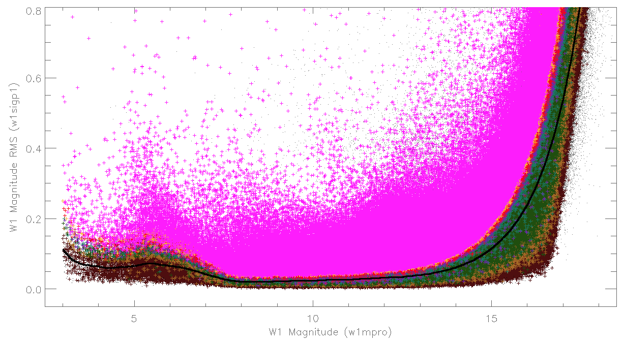
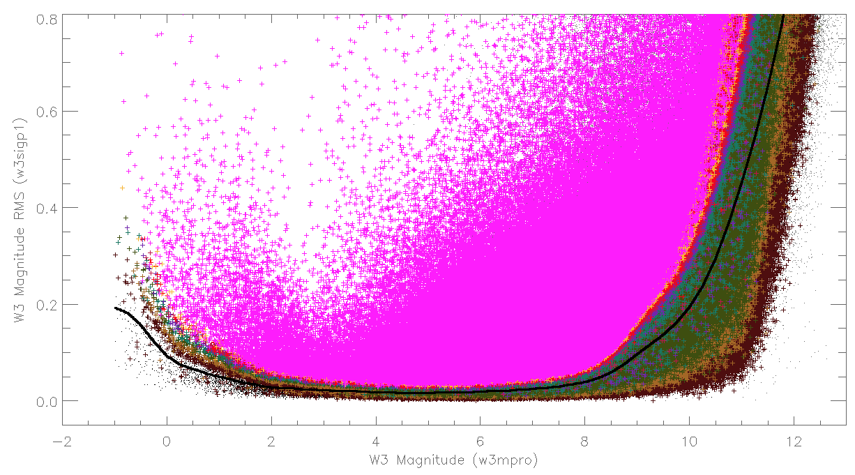
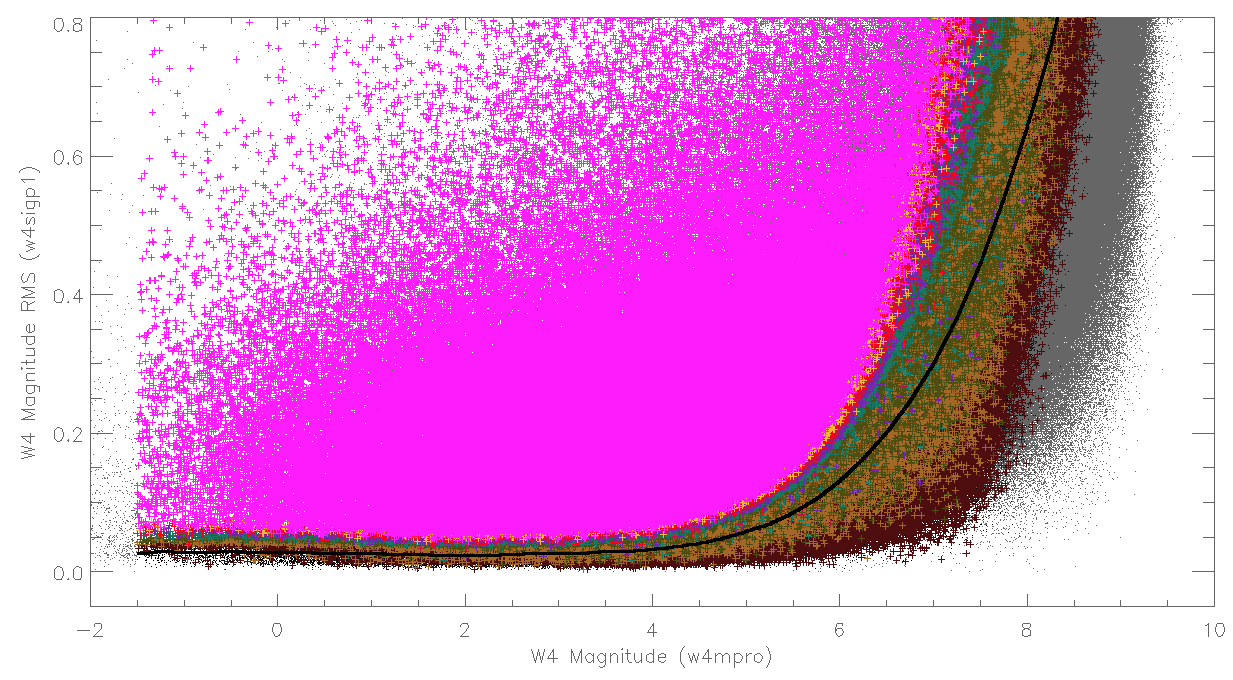
Figures 1-4 are graphical representations of the method applied to a large fraction of the sources in the all-sky release. In each plot, the values of w?sigp1 are plotted as a function of magnitude for individual sources. The small grey dots are catalog sources with F = 'n', which have inadequate or insufficient data to make a variability determination. F = 'n' sources dominate the distribution, as M ≤ 10 coverage is very common, as are artifacts, and confusion. The different colors represent different F values that are non-null, ranging from F = 0 (black) to F = 9 (magenta). Known variables are generally safely in the F = 9 region, with large amplitude variations. Sources with true variability in W3 and W4 are quite rare due to the extensive artifacts and the smaller number of total sources in those bands.

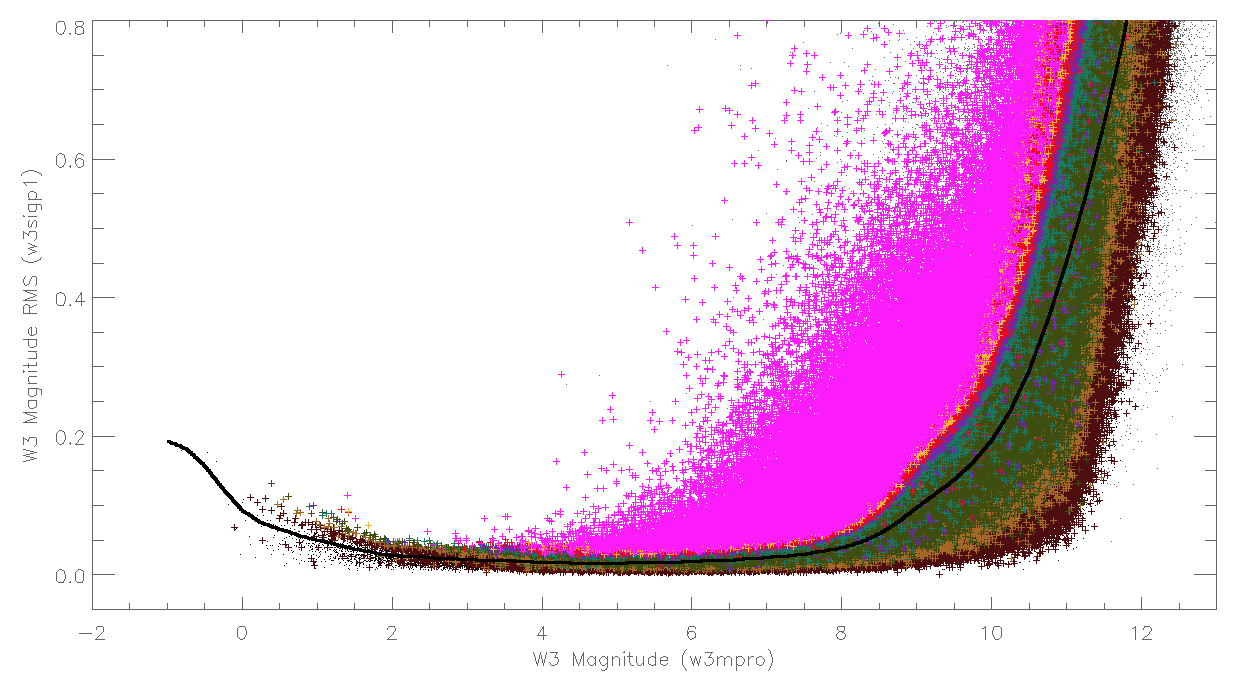
Extended sources (those with ext_flg ≠ 0) tend to have characteristics consistent with true variable sources. However, these variations are spurious, usually caused by the attempts to fit a single PSF to resolved and/or confused sources. Thus, to greatly increase reliability in use of the var_flg, one should exclude extended sources. The effect of excluding extended sources is shown in Figures 1b-4b.


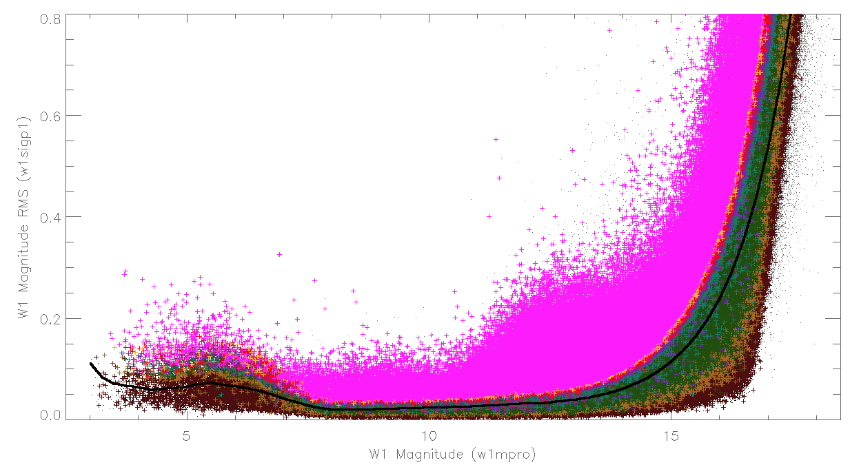Figure 1a - Plot of approximately 40 million sources from the all-sky data in band 1. Grey dots are sources with F=n. Black dots are F=0 sources. Maroon crosses correspond to low variability sources (F=1). Different colors represent different F-values to to F=9 (magenta crosses). The black solid line is the reference σ value from Equation 1.	Figure 1b - Same as Figure 1a, but excluding sources with ext_flg ≠ 0.

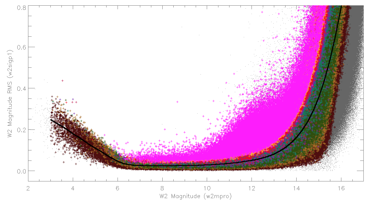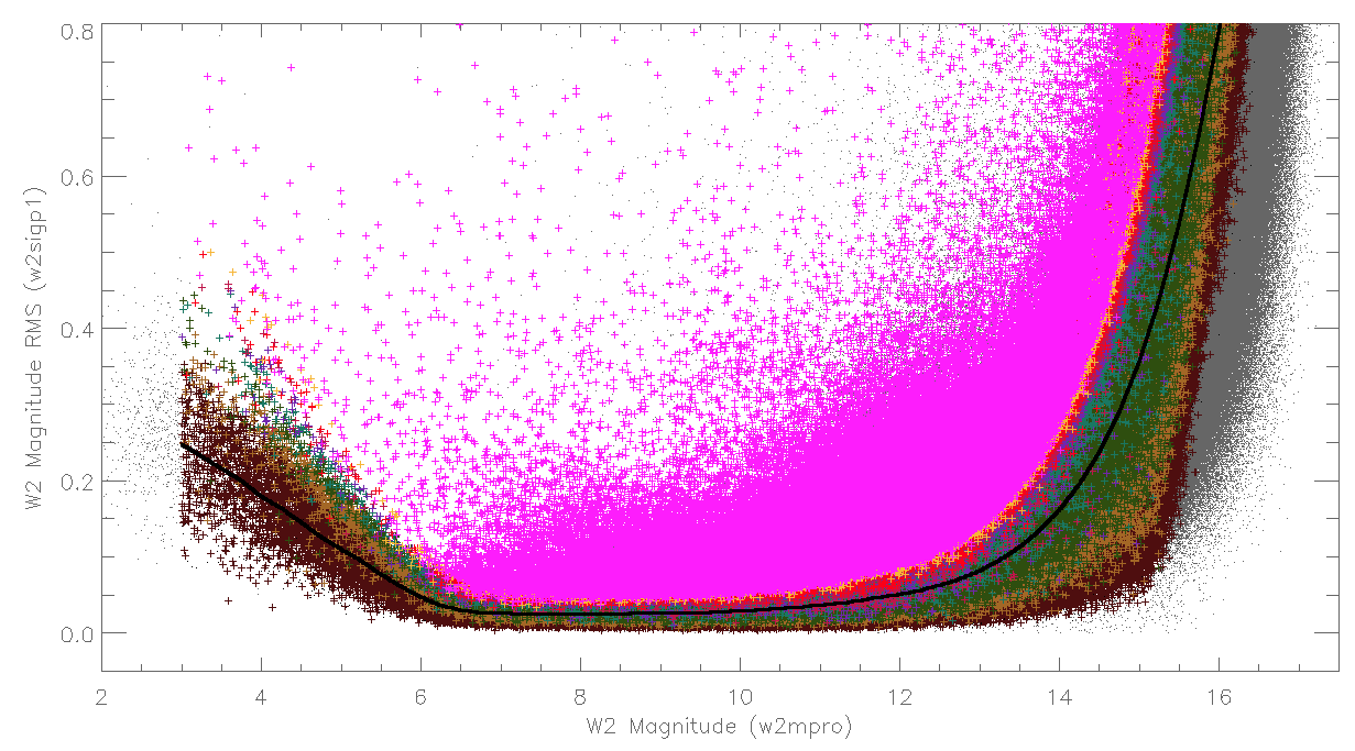
Figure 2a - Same as Figure 1a for band 2.	Figure 2b - Same as Figure 1b for band 2.

Figure 3a - Same as Figure 1a for band 3.	Figure 3b - Same as Figure 1b for band 3.

Figure 4a - Same as Figure 1a for band 4.	Figure 4b - Same as Figure 1b for band 4.

The distribution of var_flg values ≠ "n" in W1 are given in the pie diagram in Figure 5. Approximately 51.5% of the sources have F=0 and 1.5% have F=9. The total percentage of "significantly" variable sources (F > 6) that are evaluated is about 1.97%. Sources with F > 7 can generally be regarded as having a high reliability of being variable. Sources with F = 7 have approximately a 40% false-positive rate with ext_flg = 0. The total number of sources in the catalog flagged with F > 6 in at least one band is 14,163,072 (or 2.51% of all catalog sources). The number of sources with F > 6 and ext_flg ≠ 0 is 6,835,155 (1.21%). The total number of sources with var_flg = 'nnnn' is 155,946,270 (27.7%), which is comprised mostly of highly confused sources or those in regions with low depth-of-coverage.

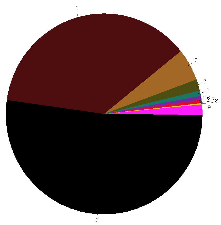Figure 5 - A pie-diagram of the fractional composition of non-null var_flg values for band 1. The values of F are labeled and the colors are the same as Figures 1a-4b.

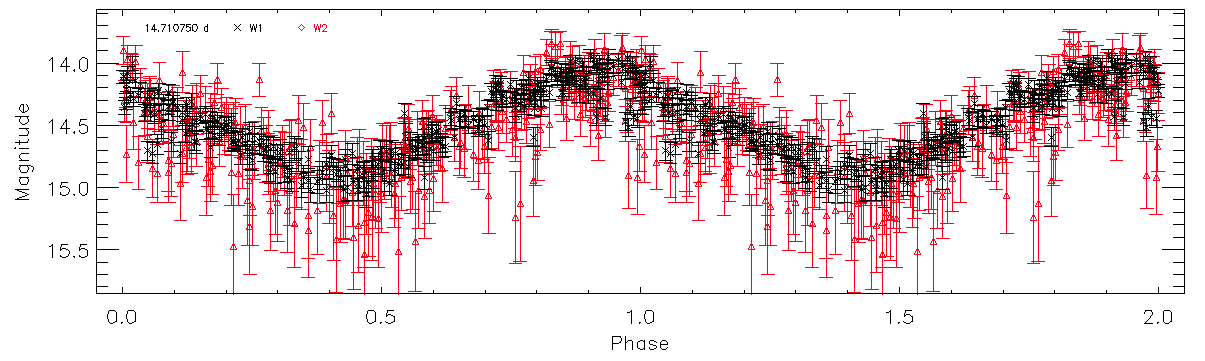
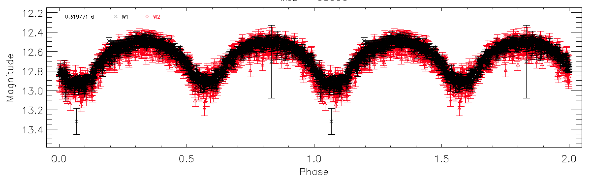
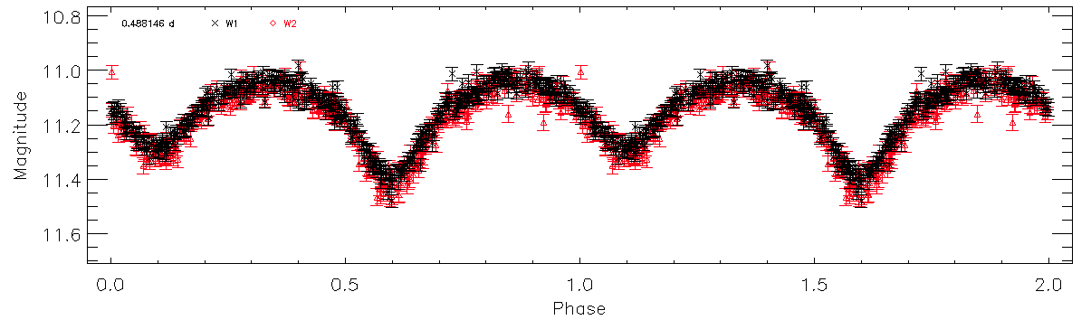
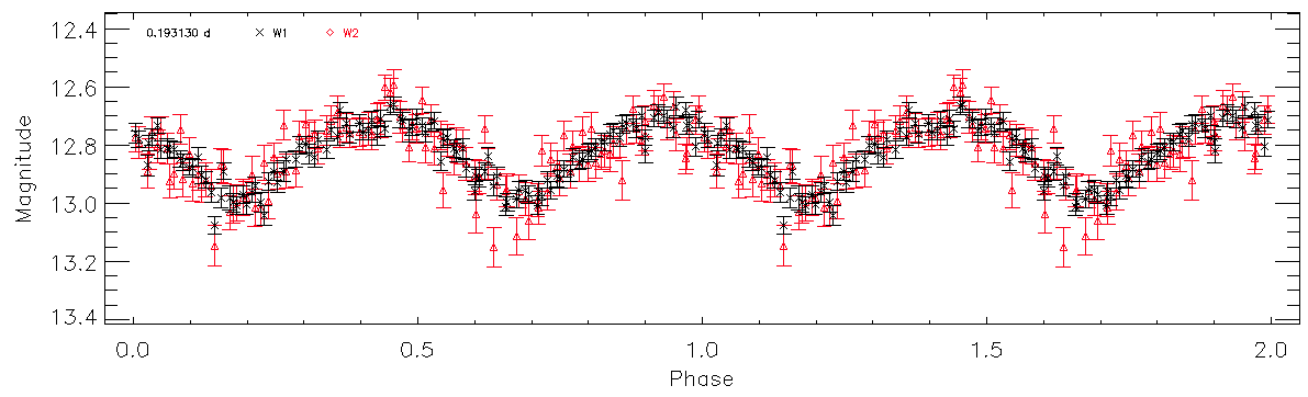
Sample WISE light curves of periodic variables that were identified using their var_flg values in W1 and W2 are shown in Figures 6-11. They are phased to the peak of the Lomb-Scargle periodogram.


Figure 6 - Phased light curve of a candidate Cepheid with a period of 14.7 days (var_flg = '99nn'). W1 data are in black, and W2 data are in red.	Figure 7 - Phased light curve of a W UMa-type eclipsing binary near the north ecliptic pole in high coverage (var_flg = '99nn').	Figure 8 - Phased light curve of the known RR Lyr variable RT Dor (var_flg = '99nn').

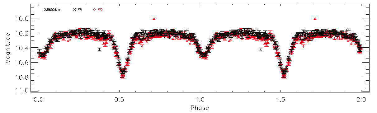
Figure 9 - Phased light curve of a β Lyr-type eclipsing binary in bands 1 and 2 (var_flg = '991n').	Figure 10 - Phased light curve of an Algol-type eclipsing binary (var_flg = '993n').	Figure 11 - Phased light curve of a candidate RR Lyr variable (var_flg = '99nn').

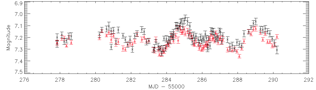
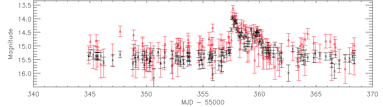
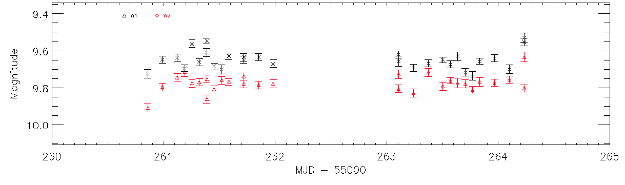
Figures 12-14 are example light curves of non-periodic variables in bands 1 and 2.


Figure 12 - The light curve of a RS CVn system with irregular features (var_flg = '9990'). W1 data are in black, while W2 data are in red.	Figure 13 - The light curve of a high-mass X-ray binary featuring a transient event (var_flg = '99nn').	Figure 14 - The light curve of the BL Lac object HB89 1749+701 (var_flg = ''9996').

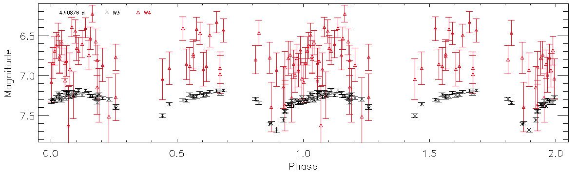
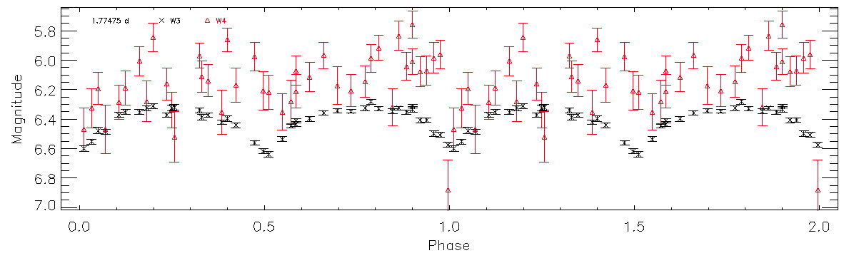
Figures 15-17 illustrate light curves of objects with variability in bands 3 and 4.


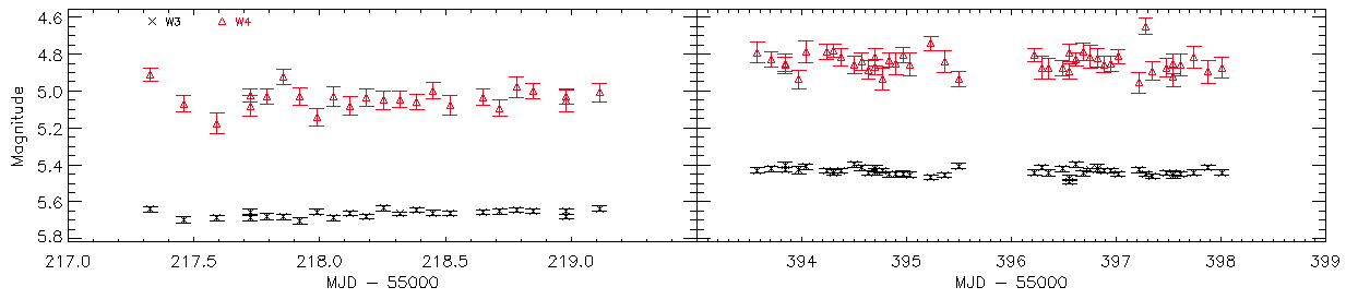Figure 15 - Phased light curve of AH Cep, a β Lyr-type eclipsing binary in W3 and W4 (var_flg = '9992'). W3 data are in black, while W4 data are in red.	Figure 16 - Phased light curve of GT Cep, an algol (var_flg = '9993').	Figure 17 - A common type of W3 and W4 variability, where the source has changed in flux during two epochs (var_flg = '9999'). This source is in the region where WISE completed two passes on the sky during the full cryogenic phase.

Figures 18 and 19 are light curves of sources with F = 7. Variability in sources with F = 7 starts to become more uncertain. While the majority of F = 7 are still variable, many of the known issues discussed in the next section start to become more common. Requiring correlation coefficients greater than 2 may help to reduce the number of flase positives in the F = 7 population.


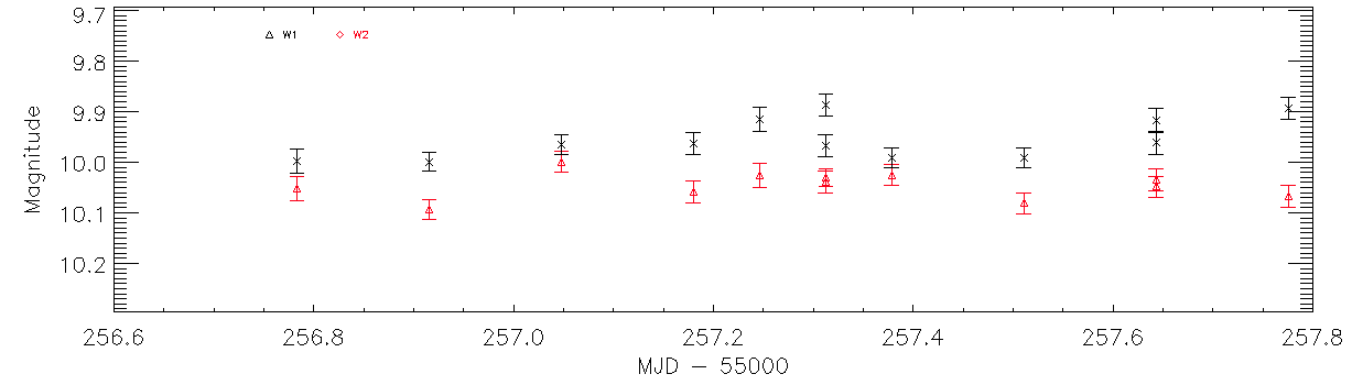Figure 18 - An example of a source with var_flg = '7711'. In this case, the correlation coefficient, q12, is 4, which is a good indication of variability, despite only a few measurements far from the mean.	Figure 19 - Another source with F = 7 in W1 and F = 3 in W2. There are subtle hints of periodic variability, but the amplitude is not high enough for positive identification.

Figure 20 is an example of a F = 1 source. 88% of flagged sources have variability flags of '0' or '1', and this is a common example of a non-variable source.

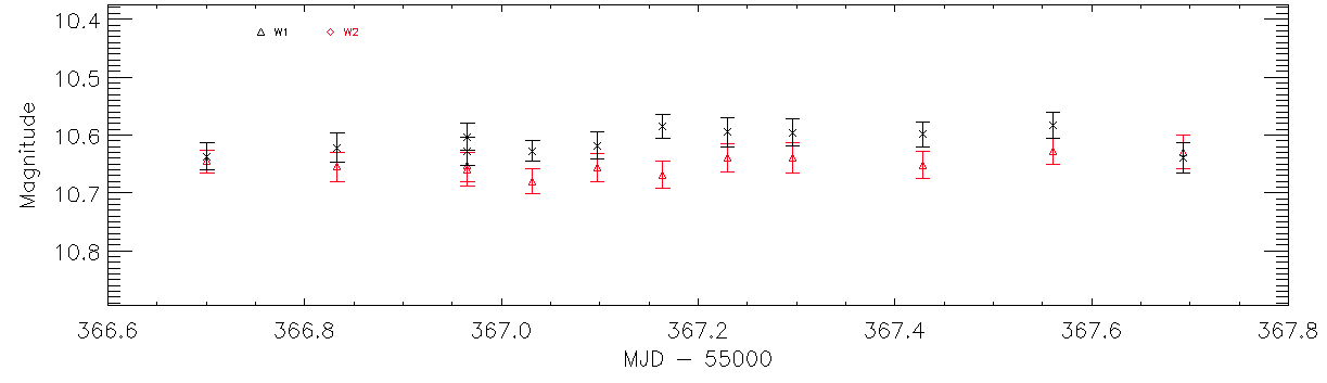Figure 20 - The light curve of a source with var_flg = '11nn' for bands 1 and 2. The source is not statistically variable during the observation period.

Sources flagged as extended and/or having contaminated artifact flags are more likely to be flagged as variable. Figure 21 is a light curve of a source flagged with var_flg = '9999', but the variability is due to contamination from the halo of a bright star. While there are many sources that have non-zero extended flags that are intrinsically variable, the false-positive rate increases for extended and contaminated sources.

Figure 21 - The light curve of a source with F = 9 in all bands, but is unlikely to be intrinsically variable. The source suffers from confusion with high rchi2 values, and has cc_flags = 'hhHH'.

Known Issues

There are some known limitations with the variability flagging algorithm that can result in anomalous var_flg values.

Nebulosity around the source can create false variability. Because the multiframe and Level 1b source locations are slightly different, the multiframe measurement of the single-exposure frames is affected by slight variations in the nebulosity intensity as each frame probes slightly different locations.

Unflagged artifacts (mostly from off-frame sources) contribute to larger than normal dispersion in the flux measurements, leading to false signs of variability.

Flagging of artifacts is sometimes too aggressive, which leads to many F=n variability flag values where light curves are generally unaffected.

Sources flagged as being real but contaminated by an artifact (cc_flags values that are lower-case letters) generally have unreliable flux measurements, and thus are more likely to be anomalously flagged as variable. Caution should be used when encountering sources flagged as both variable and contaminated with artifacts.

A close companion can increase the uncertainty in flux measurements, falsely increasing the probability of variability. This can be reduced using the constraint "na=0", but some still make it through.

Sources with ext_flg > 0 can have unreliable variability flagging due to poor PSF fitting. This is especially true in bands 3 and 4, where a large fraction of F = 9 sources are extended sources or unflagged artifacts.

The population distribution of w?sigp1 does not follow a gaussian or chi-square distribution, but is close to a chi-square. The upper-percentile cut for σ is a correction. Fainter magnitudes tend to more closely follow a chi-square distribution. See the next section for more details.

The variability probability computation is not sensitive to short-lived, low-amplitude, transient events.

Sources that are saturated can be falsely flagged as variable. This is due to inaccurate PSF matching of the wings. For maximum reliability, exclude saturated sources.

Using the Variability Flag in Searches

When incorporating the variability flag into catalog searches, remember that the flag is a string. You will likely need to use custom SQL in searches. For example, if you are using the IRSA/GATOR, search engine, search for sources with F > 7 in W1 and W2 and F > 5 in W3 by entering the following in the "Additional Constraints (SQL)" box: " var_flg matches '[8-9][8-9][6-9]?' ". In most cases, it is best to place a constraint on at least two bands to minimize the likelihood of being fooled by one of the known issues that cause anomalous variability flagging.

For maximum reliability when identifying variable sources, one should also pick sources that have ext_flg = 0. This will exclude extended sources and sources with high chi-squared values cause by confusion and unflagged artifacts. The constraint on the ext_flg is particularly important for W3 and W4 sources, as those bands experience many more artifacts. Requiring high q12/q23/q34 values also increases reliability, especially for periodic variables. Saturated sources can also have unreliable flux measurements and can be anomalously flagged as variable. Thus, constraints for a high reliability search for variables in band 1 would be: " var_flg[1] = '9' and ext_flg = 0 and q12 = 9 and w1mpro > 8 ".

Last update: 2013 February 26