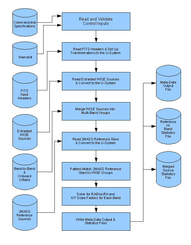
Scan/Frame position reconstruction is performed by the SFPRex module of the PRex subsystem. The processing consists of matching astrometric reference sources with WISE detections corresponding to single sources on the sky, using these matches to compute frame geometry and sky position, updating FITS headers with the improved estimates, and performing various bookkeeping functions. This processing depends on distortion calibration, which is the purpose of the gnDSTR module. Both of these depend on evaluating the effects of differential aberration, which is handled by the gndfab and diffabr8 modules. Refinement to tile position parameters is performed by the MFrefine module.
The computations performed by SFPRex are based on three primary inputs (in addition to the usual command-line and namelist control inputs).
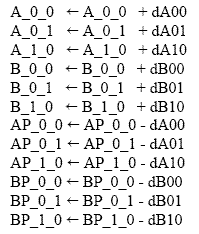
CRVAL1, CRVAL2, CRPIX1, CRPIX2, CD1_1, CD1_2, CD2_1, CD2_2, CROTA2, CRDER1, CRDER2,UNCRTPA,CDELT1, CDELT2, CSDRADEC, A_0_0, A_0_1, A_0_2, A_0_3, A_1_0, A_1_1, A_1_2, A_1_3, A_2_0, A_2_1, A_2_2, A_2_3, A_3_0, A_3_1, A_3_2, A_3_3, B_0_0, B_0_1, B_0_2, B_0_3, B_1_0, B_1_1, B_1_2, B_1_3, B_2_0, B_2_1, B_2_2, B_2_3, B_3_0, B_3_1, B_3_2, B_3_3, AP_0_0, AP_0_1, AP_0_2, AP_0_3, AP_1_0, AP_1_1, AP_1_2, AP_1_3, AP_2_0, AP_2_1, AP_2_2, AP_2_3, AP_3_0, AP_3_1, AP_3_2, AP_3_3, BP_0_0, BP_0_1, BP_0_2, BP_0_3, BP_1_0, BP_1_1, BP_1_2, BP_1_3, BP_2_0, BP_2_1, BP_2_2, BP_2_3, BP_3_0, BP_3_1, BP_3_2, and BP_3_3.
A subset of the 2MASS Point Source Catalog (PSC) serves as the primary astrometric reference for WISE position reconstruction. The astrometric reference subset, referred to as "2MRef", consists of 32,074,024 sources selected from the 2MASS PSC to have the most accurate positions. 2MRef sources satisfy the following 2MASS PSC criteria (see section II.2.a of the 2MASS Explanatory Supplement for a description of 2MASS Catalog parameters):
| 5.5 mag ≤ k_m ≤ 12 mag | 2MASS Ks brightness regime corresponding to best positional accuracy |
| k_snr ≥ 20 | High SNR Ks measurement requirement |
| rd_flag = '[12][12][12]' | Source is not saturated in any band |
| bl_flg = '111' | Source is not blended with a nearby object |
| mp_flg = '0' | Source is not confused with foreground solar system object |
| Proper motion < 0.05 arcsec/year | Proper motions taken from Bastian, U. & Röser, S., 1993, "PPM Star Catalogue", Astronomisches Rechen-Institut, Heidelberg, Høg E., et al., 2000, A&A, 355, 27 (Tycho-2), Ivanov, G.A., 2008, KPCB, 24, 334, Lepine, S. & Shara M.M., 2005, AJ, 129, 1483, and Platais, I., et al., 1998, AJ, 116, 2556. This eliminated 199,842 sources. |
SFPRex reads 2MRef data provided by a database-access utility upstream in the scan/frame pipeline and formatted into a table file containing the 2MASS PSC parameters ra, dec, err_maj, err_min, err_ang, and k_m. There are on average 446 2MRef sources per WISE frame, but actual counts vary considerably with sky position and not all 2MRef sources are detected in all four WISE bands. Proper motion corrections that would have accounted for motion in the ten years separating the 2MASS and WISE survey epochs were not applied. Proper motions are not part of the 2MASS catalog, and the requirement is to reconstruct to 2MASS.
Figure 1 shows the processing flow for the SFPRex module. This module is called by the WSDS Scan/Frame Pipeline and operates on a single frameset (i.e., a group of four single-band frames, one per wavelength channel, observed at the same sky position at the same time). Based on a discrepancy analysis of the sources observed and matched in the four channels (or fewer channels when some data are missing) and the 2MRef astrometric data, chi-square minimization solutions are obtained for five parameters in each channel: RA, Dec, Twist, SFX (scale factor in the X direction, across columns), and SFY (scale factor in the Y direction, across rows). Optical distortion (including differential aberration) is taken into account in mapping source positions from frame coordinates to sky coordinates (see section vii for a discussion of distortion calibration and section viii for a discussion of differential aberration).
 |
The SFPRex module initializes itself by:
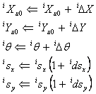
The WISE and 2MRef sources are transformed (including distortion correction for the WISE sources) into the U system. The U system is centered at the adjusted a priori center position of the shortest wavelength band in use. Its y-axis points north, its x-axis west, and its units are always arcseconds. Once the U system is set, it remains locked in that sky position regardless of any band-frame position adjustments made during the SFPRex processing.
The native coordinate system for a group of source detections in a given band is called the band-frame coordinate system or f system. This is in units of pixels and maps directly to the individual FITS images in each band. The band-frame coordinate systems for different bands do not share a common zero point, plate scale, or twist angle. In other words, each is related to the U system by five parameters:
| Xu0 | X offset in arcsec of band-frame origin from U-system origin |
| Yu0 | Y offset in arcsec of band-frame origin from U-system origin |
| θ | Rotation in degrees of band-frame axes relative to U-system axes |
| sx | X scale factor to convert from band-frame to U system |
| sy | Y scale factor to convert from band-frame to U system |
To distinguish between WISE bands, a superscript prefix i is used; e.g., iXu0 is the X offset of the band-frame origin for band i relative to the U-system origin, etc.; nominally i runs from 1 to 4. By default, distortion is corrected directly in band-frame coordinates. After that, U-system coordinates (Xu, Yu) are computed from band-frame coordinates (Xf, Yf ) in band i as follows.
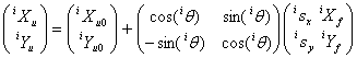 |
(Eq. 1) |
The rotation matrix in this equation will be denoted iTfu (transformation from the f system to the U system for band i) below, or just Tfu when band distinction is not needed. The goal of the subsequent processing is to match sightings of the various stars, in both 2MRef and the various WISE bands, to identify which observations apply to the same object, and to deduce corrections to the five parameters above for each band processed from the position discrepancies. The purpose of the U system is to provide a common coordinate system within which meaningful analysis of the positions of sources in different bands may be performed. The general case involves four WISE bands, and so a 20×20 system of equations is to be solved (there are also reduced systems in which certain parameters are constrained; the approach used for these will be discussed in section vi below). First the WISE detections are merged into “groups,” because even large possible telescope pointing errors should not disrupt the positions of the WISE detections relative to each other. After the WISE sources are grouped, pattern matching between them and the 2MRef sources is performed, followed by band-frame position refinement.
In order to be done optimally, the matching must take into account the uncertainties in the source positions (Xf, Yf ), where the band index i is suppressed here and for the remainder of this section to reduce clutter. The 1σ uncertainties of these coordinates in the band-frame system are σxf and σyf, respectively; the covariance between errors in these coordinates is expressed as a co-sigma, σxyf, related to the covariance Vxyf by the formula Vxyf = σxyf|σxyf|. This maintains the sign information for the correlation, since σxyf may be negative. It is more natural to carry the co-sigma along with the other uncertainties instead of the covariance because the former is in the same units as the other uncertainties. The diagonal elements of the position error covariance matrix are Vxf = σxf2 and Vyf = σyf2. The error covariance matrix is converted from band-frame coordinates to the U system via a similarity transformation as follows.
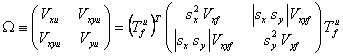 |
(Eq. 2) |
This results in the following uncertainties in the U system.
 |
(Eq. 3) |
The WISE sources are arranged into “merge groups” as follows. If only one WISE band is present, each source is taken as a “group” and used as is, i.e., the group positions, uncertainties and fluxes are those of the WISE sources. If two or more bands are present, the more general processing described below is performed.
As a first step, frame adjustment preprocessing is performed. This involves position-registering bands of wavelength higher than the lowest-wavelength band present (nominally W1) to the lowest, i.e., removing mean position offsets. The lowest-wavelength WISE band available is taken as the “seed” band, and each higher-wavelength band is processed as a “candidate” band. For each detection in the seed band, all detections in the other candidate bands are examined; if one and only one candidate detection per band is within the match radius (default 5 arcsec, specifiable on the command line via “-d”), then the match is accepted; if all candidate-band matches to the seed are unconfused (i.e., no band has more than one detection in the seed’s match area), then the position offsets are used in summations employed to compute mean candidate-to-seed offsets and RMS dispersions.
After all matching has been done for a given seed-candidate band combination, the number of matches is counted and must be at least equal to the namelist parameter MinMatch (default 3, command-line specification “-m”); if this is not satisfied, then the match radius is enlarged by a factor of 1.1 and the seed-candidate bands are reprocessed. This may be done up to 100 times, after which if it still has not succeeded, the group-merge subroutine quits and returns an error indication. If it succeeds, then the dispersions about the mean offsets are compared to the RMS seed+candidate variances for matched sources, and the former must be below a specifiable threshold. If this test fails, the seed-candidate processing is performed again from the beginning, but this time individual matches are rejected if the offset on either axis is larger than 5 times the RMS seed+candidate variance from the first pass. If all tests are passed in all seed-candidate combinations, then the mean band-to-band offsets are subtracted from the position differences used in the subsequent chi-square tests (note that the candidate-band positions themselves are not altered, since they are needed for subsequent analysis).
Note that there are no prior uncertainties for the band-to-band alignment, since these alignments are treated during IOC as too poorly known to have been modeled and after IOC as well enough calibrated to contribute no significant uncertainty relative to source extraction errors.
After frame adjustment, if any, the chi-square match testing is performed for all band combinations. Position errors are assumed to be Gaussian, and so Gaussian statistics are employed for matching and position refinement of matched sources forming a group. Groups are sought which contain one and only one source in each band, each of which passes a standard chi-square position discrepancy test with at least one other source in the group (not necessarily all), and if any source has more than one acceptable match in any other band, the entire group is rejected, and its sources may not be used in any other groups. Using the notation of Equations (1), (2), and (3) but suppressing the u subscript with the understanding that all computations here are in the U system, and attaching indexes i and j to indicate bands, and m and n to indicate detection indexes within bands, the chi-square for a pair of detections comprised of detection m in band i and detection n in band j is computed as follows. The frame-adjustment offsets in X and Y are denoted δxi and δyi, respectively; these are zero for i = 1, and all other offsets are also zero if frame adjustment has not been performed.
 |
(Eq. 4) |
Any given pair of sources in different bands is considered to have passed the chi-square test if the value of their 2-D chi-square is found to be less than or equal to the threshold chsqmx (default 6.0, which rejects 5% of all true matches and is chosen for reliability more than completeness). The numbers of confused sources and orphan sources are counted and reported in a meta-data output file.
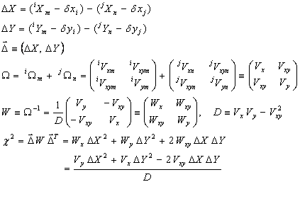
After the groups have been formed, if any, the refined position for each group is computed by normal Gaussian refinement as follows, where {G} indicates the set of band numbers represented in the group; for example, {1,2,4} corresponds to a group with detections in W1, W2, and W4. Since each band present is represented by only one detection, we suppress the detection-within-band index; e.g., iVx is the X uncertainty variance in U-system coordinates for the group’s detection in band i, whatever its detection index within that band may be.
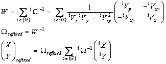 |
(Eq. 5) |
Note that if frame adjustment has been specified, the adjusted band positions are used to compute the weighted average merge group positions. This means that the merge group positions are tied to the shortest wavelength band, but have the advantage of including sources which appear only in longer wavelength bands. The flux reported for the group is the brightest of any of the sources in the group (i.e., minimum magnitude). The average offsets of the group from the seed band (lowest wavelength) are computed and reported for both axes.
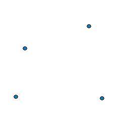
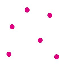
The pattern matching algorithm uses “separation bar” matching to identify potential star pairs common to 2MRef and the WISE groups. Figures 2 and 3 illustrate a simple case involving four 2MRef stars and six WISE merge groups, respectively. In practice, not all 2MRef stars and WISE groups are used; the depth is determined by the ldepth parameter, which defaults to 99, meaning that only the brightest 99 2MRef and WISE groups are used.
 |
 |
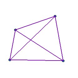
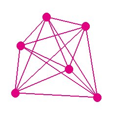
Each 2MRef star used for pattern matching is connected to each other one by a “separation bar”, as shown in Figure 4; the same is done for the WISE merge groups, as shown in Figure 5. Each bar is characterized by a slope and a length. The location of the endpoints is not considered significant, since the point of this analysis is to discover rather large offsets between the 2MRef and WISE patterns. The goal is to identify which separation bars are the same for the two groups of stars, as illustrated in Figure 6. For this simplified example, all the 2MRef separation bars also show up as WISE separation bars. In general this will not be the case.
 |
 |
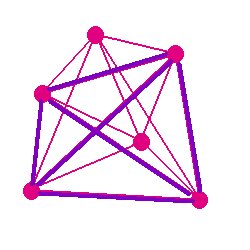 |
For N stars (of either type), there are N(N-1)/2 separation bars (i.e., the same as the number of elements above the diagonal of a matrix). All such bars are processed by computing the slope and length and recording the ID numbers of the sources at both ends of the bar. In order to be usable, a bar must have a length of at least sepmin (default 60 arcsec). The parameters for sufficiently long bars are stored in arrays to produce two sets of data, one for the 2MRef reference stars and one for the WISE groups. The stars defining the endpoints of the bar are stored with the one closest to the center of the array first; this is done so that endpoint star pairings between 2MRef and WISE may be assumed later to be such that the first entries correspond to each other and the second entries correspond to each other (the very small fraction of cases in which position errors invert this relationship are neglected and simply drop out of consideration).
Slope and length matches between these two data sets are then sought by considering each point in one data set in combination with each in the other as follows.
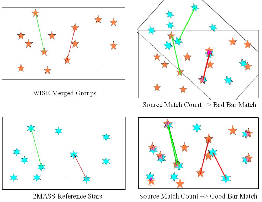 |
Upper left: WISE sources Lower left: 2MASS sources. Green bars are a correct match, red bars are not. Upper right: Forcing red-bar alignment produces few good source pairings Lower right: Green-bar alignment yields many pairs |
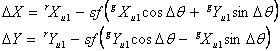
The procedure for matching the pattern of 2MRef reference stars to the WISE groups (bandmerged WISE detections) involves evaluating each candidate separation bar match by forcing the end points of the WISE bar to match those of the corresponding 2MRef bar exactly. This is done by computing the translation (ΔX and ΔY), rotation (Δθ), and rescale factor (applied to both axes) sf that make this happen. This section provides the mathematical details of this computation and the error analysis for the parameters computed.
Figure 4 shows the separation bars that are defined between all 2MRef reference stars relative to each other. Figure 5 shows the same information for the WISE group sources. Each bar in the WISE set is compared to each bar of approximately the same length in the 2MRef set as follows: if we assume that the two WISE sources are observations of the two 2MRef sources, does forcing the two separation bars to lie exactly on top of each other cause a significant number of other alignments between WISE sources and 2MRef counterparts? By “alignment”, we mean that the coordinates of a WISE group source lie within a small radial distance from the coordinates of a 2MRef source.
To test this hypothesis for a given pair of separation bars (one WISE bar and one 2MRef bar), we compute a transformation that makes the two WISE source coordinates equal to the corresponding two 2MRef source coordinates, and then we apply this transformation to all the WISE sources. Then we attempt to match the two source lists and count the number of matches. Note that these matches are done considering all sources in both lists, not limited to the ldepth brightest sources as was the case for separation bar matching.
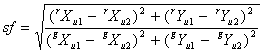
All source coordinates are in the U system. The WISE group sources will be denoted with a superscript prefix g, the 2MRef reference sources with an r, and the two sources of each type will be distinguished with subscripts 1 and 2 following the u designating the U system. For each WISE-2MRef source pair defining the bars, we have a coordinate transformation similar to Equation (1) that converts the WISE coordinates to the same values as the 2MRef coordinates: translation by ΔX and ΔY, multiplication by a scale factor sf, and rotation by an angle Δθ. Since the four pairs of source coordinates are all known, the values of these four parameters can be found by solving the four equations in four unknowns formed by the two vector equations for the transformation:
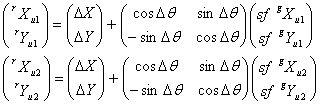 |
(Eq. 6) |
The equations are nonlinear in Δθ, however. We will get around this by treating the sine and cosine as separate variables, making five unknowns, and adding a fifth equation:
 |
(Eq. 7) |
The ratio of bar lengths gives the scale factor value directly; this can then be treated as known in Equation (6), and the values of ΔX, ΔY, sinΔθ, and cosΔθ could be obtained by standard solution of a 4×4 linear system, after which Δθ could be found by computing the inverse tangent of sinΔθ/cosΔθ. It is not necessary to do this as part of a full 4×4 linear system, however, because Δθ can be found directly as follows; we define the following vector representations of the WISE and 2MRef separation bars:
 |
(Eq. 8) |
These vectors have the same length, because the second is just the 2MRef bar expressed as a vector with its magnitude divided by sf. Disregarding their origins, the only difference between these two vectors is their orientation, which differs by the angle Δθ. Rotating the WISE bar vector by Δθ would make it equal to the 2MRef bar vector:
 |
(Eq. 9) |
Carrying out the multiplication yields the 2×2 linear system
 |
(Eq. 10) |
The solutions for sinΔθ, cosΔθ, and Δθ are
 |
(Eq. 11) |
Now ΔX and ΔY can be obtained from either vector expression in Equation (6):
 |
(Eq. 12) |
Assuming that ΔX and ΔY are within acceptance tolerances, the transformation in Equation (6) can now be carried out on all the WISE group sources, and then a matching of WISE and 2MRef sources can be attempted, and the number of successful matches counted. To be successful, one and only one WISE source must lie within a 2MRef source’s acceptance region. The probability that all such matches are due to random coincidence is computed and must be below a maximum value mxpran (default 1.0e-8), or else the bar match being investigated is rejected. This probability is based on a Poisson model, for which the probability of N sources falling randomly into the match-acceptance area, given that the mean number of random sources in that region is λ, is
 |
(Eq. 13) |
In this case, λ depends on the local WISE group source density, since the matching is done by searching the WISE source list for matches to each 2MRef source. Thus the source density is determined by WISE, and the total area for random matches is the number of 2MRef sources multiplied by the match-acceptance area per source. The WISE source density is taken to be the number of WISE sources divided by the area being processed, where the latter is the rectangular area defined by the minimum and maximum X and Y coordinates expanded by the match acceptance distance. The total acceptance area is the area within a circle of radius drwin multiplied by the number of 2MRef sources. λ is the product of the local WISE source density and the total match acceptance area. Given N matches found, not counting the two that defined the bar alignment, Equation (13) gives the probability that they are all random.
The correct registration of the WISE and 2MRef source patterns generally can be found by any number of bar matches, as is obvious from the fact that to be successful, a bar match must produce some other WISE/2MRef associations, and these other associations have their own bar matches that should also yield the same basic pattern match. Since these other sources have their own independent position errors within their respective coordinate systems, they contribute independent information to the solution for ΔX, ΔY, Δθ, and sf which may be averaged (although some accounting for the correlation between two bar matches sharing a common source pair must be made; see section iv.3 for details). Whether averaging is done is controlled by the useals parameter (default T). The best pattern match is that which produces the largest number of WISE/2MRef associations. This count may be produced by more than one bar match, and all that yield the same maximal number of associations are eligible to have their solutions averaged.
For use in averaging and outlier rejection, as well as for
downstream purposes, the uncertainties associated with the four parameter solutions for a given
bar match are needed in the form of a full 4×4 error covariance matrix, and so we will describe
how these are calculated. Each of the four parameters is a function of the same eight variables, the four source coordinate
pairs. We will define a vector  composed of the four parameters
and a vector
composed of the four parameters
and a vector  composed of the eight coordinates.
 |
(Eq. 14) |
We wish to construct the error covariance matrix for ,
which we will call Ω.
 |
(Eq. 15) |
The ε variables are the errors in the parameters indicated by their subscripts. By using derivatives to compute the dependence of the four-parameter errors on the source coordinate errors, we are assuming that the latter are small enough to ignore second-order terms. We also treat the source-coordinate errors as uncorrelated, because the WISE source extraction algorithm did not compute the covariance between X and Y coordinates when this algorithm was coded, and ignoring it here constitutes a conservative calculation. It could always be included by keeping the corresponding cross-terms in the expectation values in the last line of Equation (15), as follows:
 |
(Eq. 16) |
The covariance matrix for the errors would
have to be provided as input. This is not
anticipated, since it would be mostly zeroes off of the diagonal; the errors in one source’s
coordinates are uncorrelated with those of a different source to a high degree of approximation,
and only fairly weak X-Y correlations for individual sources would exist.
The 32 partial derivatives in the third and fifth lines of Equation (15) (four parameters with eight derivatives each) are obtained by using Maple’s differentiation operator with the equations defining the functional dependence of the four parameters on the eight position coordinates. The elements of the error covariance matrix are then evaluated as shown on the last line of Equation (15). The summations in Equations (15) can be represented in vector-matrix format as follows.
 |
(Eq. 17) |
The computations described above are generally done for several dozen to several hundred bar
matches, each yielding its own and Ω.
We will subscript these with n to indicate a single vector
and error covariance matrix, n = 1 to N, the number of
bar matches found usable by virtue of
tying for the maximal number of 2MRef/WISE matched sources. These solutions are then
averaged using inverse-covariance weighting as follows.
 |
(Eq. 18) |
The position coordinate errors are believed
to be well approximated as Gaussian, and since the
errors are linear combinations of
the errors, by the Central Limit Theorem, they should be
Gaussian to an even higher degree of approximation. This justifies the use of Ω for
inverse-covariance averaging. Once the average parameter vector is
obtained, chi-square is computed for each bar match.
 |
(Eq. 19) |
The error covariance matrix for the average is subtracted from that for the data as a result of the fact that the errors in the data and the average are correlated. The chi-square per bar match has 4 degrees of freedom, being composed of a 4-vector with the mean of each component subtracted off. A second average is computed in the same way as shown in Equation (18) except that any given solution is rejected if its chi-square value is greater than ChSqMx4 (default 10, which rejects 4% of all true chi-square samples with 4 degrees of freedom).
The sum of the chi-square values over all retained solutions is computed; this chi-square would have 4N’ degrees of freedom, where N’ is the number of solutions retained in the second averaging, if all sources used in bar matches were distinct, i.e., if each source participated in only one bar match. This is not generally true, however, since as Figure 6 shows, a given source may be an endpoint of more than one usable bar. The presence of a given source in more than one bar-match solution introduces correlations which make the uncertainty computed in Equation (18) an underestimate. To ignore this would generally result in an unacceptable error, but a detailed accounting would require a 4N’×4N’ covariance matrix, most elements of which would be zero. Instead of a detailed and expensive computation of the effects of duplicated bar endpoints, an approximate compensation factor is computed as follows. A search of the reference source positions is undertaken to identify duplications in bar matches retained for the final solution. For each duplication, 2 degrees of freedom are deducted (since one reference source and one WISE source were duplicated). If there were no duplications, the number of sources (WISE and reference) used in the final solution would be 4N’. With K sources found in a sequential search of the reference sources to be involved in a retained bar-match higher up in the list, the number of degrees of freedom drops to M = 4N’-2K. The error covariance matrix elements for the final average are scaled by 4N’/M to compensate approximately for the correlations.
The value of QM(χ2total) (the fraction of all chi-squares with M degrees of freedom above the observed total chi-square value) must be greater than Qmin4 (default 0.001) or else the final uncertainties must be inflated, as follows.
 |
(Eq. 20) |
In other words, the elements of the error covariance matrix are scaled to yield a chi-square of nominal value.
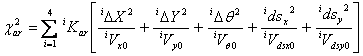
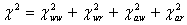
Each source pair matched by the above processing is used to compute position discrepancies which contribute to summations of chi-squared values. These total chi-squares are then minimized by solving for corrections to the 20 parameters, i.e., the five per band listed in section ii. There are also a priori estimates of all 20 parameters and their uncertainties. Band-to-band and absolute relationships are included via proxy “measurements”: three artificial sources “observed” in each band, that serve to constrain band-to-band changes, and terms that constrain absolute changes (i.e., changes involving the band-to-band relationships remaining constant but all parameters changing the same way in each band). While the total chi-square summation depends on the 20 parameters, it is convenient to split it up into four components: χ2ww, the part depending only on discrepancies between pairs of matched detections in different WISE bands; χ2wr, the part depending only on discrepancies between pairs consisting of a single-band WISE detection matched with a 2MRef source; χ2aw, the part depending only on discrepancies between pairs of “matched” proxy detections in different WISE bands; χ2ar, the part depending only on absolute changes to the 20 parameters. In each band, we write each of the five coordinate transformation parameters in Equation (1) as a sum of the current estimate for that parameter and a correction; the goal is to solve for these corrections by finding the values that minimize the total chi-square summation.
 |
(Eq. 21) |
When these substitutions are made in Equation (1), the coordinates obtained in the U system become explicit functions of the five correction parameters. The first three are absolute correction factors indicated by the character Δ; the last two (for the scale factors) are relative correction factors indicated by the character d. The first chi-square summation is as follows.
 |
(Eq. 22) |
This summation extends over all pairs of bands i and j, and within those bands, all pairs of detections n and m, respectively. The number of detections in bands i and j are Ni and Nj, respectively. The quantities summed are the individual chi-squares corresponding to the differences between each source pair’s U-system X coordinates and Y coordinates, i.e., the products of all pair combinations of the coordinate differences weighted respectively as indicated by Wx, Wy, and Wxi, each with band prefixes i and j and source-number-within-band suffixes n and m. The weights are zero for all source pairs that are not matched; this implies also that the weights are zero for any pairs involving bands that are not being processed. For a pair of sources which are matched,
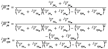 |
(Eq. 23) |
where we have attached band prefixes and source-number-within-band suffixes to the uncertainty variances Vxu, Vyu, and Vxyu defined in Equations (2) and (3). These expressions result from expanding the chi-square for a full error-covariance matrix (i.e., nonzero off-diagonal element) in a manner analogous to Equation (4). Note that in the code, these summations are not actually carried out over all possible combinations as shown above; only the terms with nonzero weights are evaluated, and these are known from the group information which is stored in an array of detection pointers for each group. Similarly, an array of 2MRef associations with groups is maintained and used to evaluate the nonzero terms in the summation for the corresponding chi-square, where Nr is the number of reference stars.
 |
(Eq. 24) |
The a priori constraints represent prior knowledge of the 20 parameters; they dilute the effects of any outlier measurements that may get through the filters, and they guarantee that the system of equations will be nonsingular by assuring that some measurement exists for every parameter. The a priori band-to-band constraints are implemented via three well spaced pseudo-sources defined in the band-frame coordinates of W1 at the following locations, where the index p denotes a “pseudo” or “prior” source.
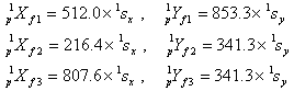 |
The a priori estimates of the 20 parameters can be used to map these three proxy sources from the W1 band-frame coordinates above to the U system for the case being processed. From there, the coordinates in the other three WISE bands can be computed, again by using the a priori estimates of the 20 parameters. The result is three pseudo-groups, each with pseudo-detections in all bands. The third chi-square can then be written in a form analogous to Equation (22), noting that these proxy sources are not coupled in any way to real WISE detections or 2MRef references.
 |
(Eq. 25) |
The factor jiKaw takes on the values specified by the namelist parameter mwm2m0, an array of values for the given combination of i and j; these allow the weighting of the a priori constraints to be adjusted if necessary. The number of proxy sources is taken to be three because that is the minimum number needed to define all 5 parameters in each band. The intent was that the weights be small enough that proxy sources never come into significant play unless WISE:2MRef match counts are anomalously low; in which case they can prevent the equations becoming singular. This adjustment factor allowed the possibility of tweaking the weights to achieve that end, after some experience had been obtained with real data. In practice, the capability was never needed and all the multipliers were left at their initial values of 1.0.
The fourth chi-square summation constrains absolute changes to the 20 parameters and is written explicitly in terms of them.
 |
(Eq. 26) |
The iKar factor corresponds to the namelist parameter mwtfp0, an array of values for each band; these allow adjustment of the relative weighting of these constraints. It was not found necessary to change these from their initial values of 1.0. The total chi-square is now:
 |
(Eq. 27) |
The substitutions in Equation (21) are made formally in Equations (1) and (22)-(26), and then the 20 derivatives are taken with respect to the 20 fitting parameters (the five corrections shown in Equation (21), one set each corresponding to (Xu0, Yu0, θ, sx, sy) for each of the four WISE bands, hence 20 correction parameters).
 |
(Eq. 28) |
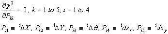
With small-angle approximations for trigonometric functions of the angle corrections, and with second-order terms in the other corrections dropped, this produces a linear system of 20 equations in 20 unknowns which is solved with standard methods. For convenience, we remap the two indexes on the fitting parameters into one dimension, n = 5(i-1)+k. Then Equation (28) becomes
 |
(Eq. 29) |
Expanding the squares in the definitions of the chi-square summations results in cross-terms in the five parameters per band, and then taking the derivatives as shown in Equation (29) produces the 20 equations in 20 unknowns which can be represented in vector-matrix form as Ax = b, where the components of the x vector are Pn, n = 1, 20, each row of the A matrix consists of the coefficients of Pn in the corresponding equation, and the b vector components are the constant terms in the 20 equations. The linearized system can be solved in a variety of ways, but the simplest method is to invert the A matrix, since that inverse is needed later anyway. Therefore we have x = A-1b. The error covariance matrix expressing uncertainties in the 20 fit parameters is just the inverse of the coefficient matrix, ΩP = A-1, where the elements of ΩP are denoted VPij, the error covariance for parameters Pi and Pj. Thus √VP11 = σ(1ΔX), V23 = cov(1ΔY,1Δθ), etc.
It is sometimes useful to constrain one or more parameters in the chi-square minimization fit, resulting in a reduced set of simultaneous equations. Within PRex, two different types of constraint are available. First, a subset of the nominal fit parameters can be selected as fixed, meaning that they will be frozen at their a priori values. Second, the fractional scale changes (dsx and dsy) within any band frame can specified to be the same. The capability to fix all parameters except for the W1 parameters 1Xu0, 1Yu0, and 1θ, (thus keeping all scale factors and band-to-band relationships constant because they had been well calibrated) was used for all processing affecting the data products. SFPRex was also run in the full 20-parameter fit mode to track possible parameter changes, but its solutions did not effect data products..
In order to fix user-specified parameters, the rows in the matrix equation Ax = b associated with those fixed parameters are dropped. The columns in the A matrix corresponding to the fixed parameters are multiplied by the fixed parameter values, then moved across the equal sign to be subtracted from the b vector. As a simplified example, consider a single-band case resulting in the following matrix equation:
 |
(Eq. 30) |
Assume it is desired to fix dsx and dsy at their a priori values dsx0 and dsy0; the reduced matrix equation becomes:
 |
(Eq. 31) |
Forcing the X and Y scale changes to be equal (solving for ds ≡ dsx = dsy) can be achieved by adding the rows and the columns associated with scale changes. This will reduce the set of simultaneous equations by one for each band where this option is selected. As an example, consider once again the single-band case, which now becomes:
 |
(Eq. 32) |
Herein the term "distortion" is used in its more general sense to include any departure of the performance of an optical system from the predictions of paraxial optics. We will, however, need to distinguish between distortion due to differential aberration (which will be referred to as "DAb distortion") from that due to all other causes (which will be referred to as "Non-DAb distortion" or just "distortion"). As will be discussed in detail later, the DAb distortion changes rapidly with time, whereas Non-DAb distortion does not. Distortion model coefficients, which are the sum of Non-DAb and DAb contributions, are input to, but never modified by, SFPRex itself. Non-DAb distortion is calibrated by the gnDSTR program using the RvB output files generated during previous SFPRex runs; these are adjusted by the gnDSTR subroutine gndfab to remove DAb effects before being used for Non-DAb distortion calibration. Modifications to the distortion coefficients due to DAb for a given frame are computed by the diffabr8 module and applied near the beginning of the scan-frame pipeline using known spacecraft velocity and telescope look direction data. This allows the complete distortion corrections to be used by all downstream processing (including SFPRex) without having to be concerned about static vs. time-dependent effects.
Each RvB file contains the associated 2MRef and WISE sources that were used to reconstruct the positions, orientations, and scale factors of the frames in each band for a single photometric integration time, along with associated position uncertainties. The WISE source positions are given in frame (X,Y) coordinates where they were extracted, and the 2MRef sources are mapped into these coordinates from their catalog (RA,Dec) positions assuming perfectly linear optical mapping based on the current knowledge of the scale factors. Any error in these scale factors is corrected by the linear terms in the distortion polynomial, which is a complete 4th-order polynomial in X and Y.
Differential aberration refers to the spatial variation of velocity-induced aberration over the focal plane. Because the relationship between the telescope line of sight and the spacecraft velocity vector varies with time, differential aberration is also time-varying and must be removed in order to calibrate the Non-DAb distortion. This is done by computing the differential aberration at the position of each WISE source and subtracting it from the position coordinates. This effect amounts to a scale change and is maximal in the corners of the array with a value of about 0.2 arcsec. Once the static (Non-DAb) distortion has been calibrated and represented as SIP coefficients in the FITS headers, each frame's SIP coefficients are individually modified as part of scan-frame pipeline initialization to add in linear SIP coefficients peculiar to that frame's differential aberration, yielding that frame's unique set of SIP coefficients. For the remainder of this section, the term "distortion" will refer to Non-DAb distortion.
The WISE and 2MRef positions for a given matched pair are generally different because of the distortion affecting the former. These differences are what the distortion polynomial fits. All the RvB files from a large number of scans are used in a single calibration in order to gain stability against the extraction errors.
Pre-launch analyses determined that a 3rd-order polynomial could not quite guarantee meeting the project requirements on astrometric accuracy, whereas a 5th-order polynomial yielded no better fit than a 4th-order polynomial. Flight data confirmed these conclusions, and it was found that the residuals in the fitting were dominated by the PSF partition model used for source extraction (PSF template fitting was done with array-location-dependent PSFs in order to meet the astrometric and photometric requirements in the context of nonisoplanatic images). The maximum residuals were smaller than the required accuracy by about a factor of 5, and so although they were systematic and significant, they were not a concern and were to be expected.
The two axes each have their own polynomial, and these were originally coupled through a skew parameter. It was found that including skew did not improve the accuracy of the model, and so skew was later forced to be zero. F2S (Frame-to-Sky) and S2F (Sky-to-Frame) models are both computed, i.e., conversion from distorted coordinates to undistorted coordinates and vice versa. Thus there are four equations whose coefficients must be computed, two F2S equations covering the “frame” X and Y axes, and two S2F equations covering the “sky” X and Y axes. The “sky” and “frame” coordinates are Cartesian systems corresponding to the same tangent projection but differing only in whether distortion operates. Each of the four equations has the same form but different coefficients. For illustration, we will consider only the F2S equation for X; the distortion on the frame X axis is denoted du. For a general Nth-order polynomial:
 |
(Eq. 33) |
The distortion on the Y axis is denoted dv, the polynomial has the same form, but the coefficients in the polynomial corresponding to Equation (33) are denoted bnk. The S2F conversions have similar forms. Given that N = 4, each equation has 15 coefficients. Since X and Y can refer to axes in either sky or frame coordinates and to WISE detections or 2MASS sources, the following notation is used to keep the various combinations distinct:
| u | X position of WISE detection in band frame (pixels, not corrected for distortion) |
| v | Y position of WISE detection in band frame (pixels, not corrected for distortion) |
| du | distortion adjustment along X axis (pixels) |
| dv | distortion adjustment along Y axis (pixels) |
| xr | reference star undistorted position in band frame along X axis (pixels) |
| yr | reference star undistorted position in band frame along Y axis (pixels) |
| xm | distortion-corrected WISE star position in band frame along X axis (pixels) |
| ym | distortion-corrected WISE star position in band frame along Y axis (pixels) |
| β | skew angle, assumed to be small (rad), later forced to zero |
The (xr, yr) coordinates are obtained by transforming the 2MRef celestial coordinates into band-frame pixel coordinates assuming no distortion exists, i.e., transforming according to frame center offsets, frame rotation, and scale factors only. If there were indeed no distortion, then these would be the expected coordinates for the matching WISE detection, (u, v). Correcting the latter for distortion yields (xm, ym), which then are the expected 2MRef coordinates. The distortion correction including skew has the following form, where skew is arbitrarily assigned to the Y axis (either axis can be used as long as skew is treated consistently throughout).
 |
(Eq. 34) |
Because of source position errors in both 2MRef and WISE, (xr, yr) and (xm, ym) are generally not equal for each given matched pair of 2MASS/WISE sources. The ank coefficients are determined via chi-square minimization of this discrepancy. For each matched pair, the position error covariance matrices are added to obtain the expected error covariance matrix for the difference, and this supplies the weights used in the chi-square minimization.
 |
(Eq. 35) |
The chi-square to be minimized is
 |
(Eq. 36) |
where the summations are taken over all matched pairs of 2MRef and WISE sources in the RvB input. The derivatives of chi-square with respect to du, dv, and β are taken formally, using Maple. Since du and dv are explicit functions of the ank and bnk (as seen in Equation (33) for du), derivatives of chi-square are actually taken with respect to the ank and bnk, and so the number of equations obtained is equal to the number of coefficients. This forms a linear system of equations for the ank and bnk given any value of the skew. Including the skew derivative equation would result in a nonlinear system, and so instead, skew was initially obtained iteratively by assuming a value to be used in the linear system, which can be solved without iteration. Once the ank and bnk were obtained, they could be used in the skew derivative equation, which was set to zero, and a solution for β was obtained. This could be used in another solution of the linear system, after which another value for β was obtained, and this process could be repeated until the β value converged. In practice, it was found that the solution oscillates, and so a damped convergence was used, i.e., each iteration used a value for β that was the average of the solutions for the two previous iterations. This was found to converge to better than single precision in only a few iterations . The skew was assumed to be zero for the first iteration, and its solution was always very small and had no impact on reducing residuals, and this led to the decision to force it to zero.
The iterative approach was retained, however, so that outlier rejection could be performed on the second pass based on large discrepancy relative to the first-pass solution. This was done as follows. After the first iteration was performed, another iteration can employ the estimates of the previous iteration to compute a chi-square contribution for each source pair, i.e., Equation (36) without the summation symbols. This yields a chi-square value with two degrees of freedom; this value must be less than the threshold ChSqMax. The default value is 8, which implies that the expected fraction of the non-outlier population rejected as outliers is 1.83%.
The uncertainties of the fit coefficients are obtained as follows. The linear system can be expressed in matrix form, where the matrix elements are the coefficients of the ank and bnk. The error covariance matrix for the estimated values of the ank and bnk is the inverse of the coefficient matrix. Tests with Code V data showed what is normally to be expected, that the errors in the ank and bnk estimates are strongly correlated. This means that a realistic estimate of the uncertainty of the distortion model needs to take the entire error covariance matrix into account. Monte Carlo studies showed, however, that with one million or more RvB pairs included in the computation, the formal uncertainties became completely negligible relative to other uncertainties in computations that depend on the distortion model (e.g., ordinary pointing reconstruction for individual frames). This data volume was achieved even in W4 and greatly exceeded in the other bands. Data from five equally spaced 5-day periods of the cold mission were used, running from IOC (In-Orbit Checkout) to just before the end of the cold mission (Julian dates 2455210-2455215, 2455260-2455265, 2455310-2455315, 2455360-2455365, and 2455410-2455415). The number of RvB pairs used were as follows.
| Band | Number of RvB Pairs |
|---|---|
| W1 | 28,838,319 |
| W2 | 29,068,502 |
| W3 | 11,105,144 |
| W4 | 1,145,346 |
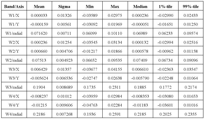
Even with only about 10% as many RvB pairs as W3, the formal W4 uncertainties turned out to be comparable in magnitude. In W1 and W2, the formal model uncertainties on each axis are 10±5 milli-arcsec; For W3, they are 6±3; for W4, they are 15±7. These are significantly smaller than the fitting residuals, which as stated earlier, were clearly dominated by the PSF partitioning.
Distortion is handled in the WISE pipelines via standard SIP coefficients in FITS headers. The ank and bnk coefficients are mapped directly into these SIP coefficients.
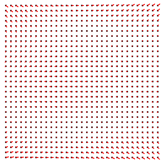
The distortion models are qualitatively similar in all bands and also to the Code V model once the rotational orientation of that model is established. In Figure 8 below, we show each band's model as a vector-flow diagram, with the vectors scaled 10×. The vectors are placed at 31×31 uniformly spaced distortion-free points in the array. The directions show how distortion moves those points to their apparent locations. The maximum vector lengths are 2.241 pixels (6.162 arcsec), 2.343 pixels (6.443 arcsec), 2.308 pixels (6.347 arcsec), and 0.931 pixels (5.120 arcsec) for bands W1 through W4, respectively.
 |
 |
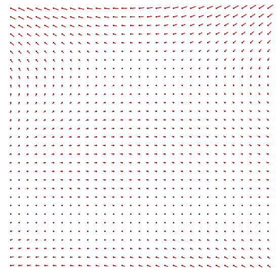 |
 |
The statistical distributions of the fitting residuals are shown in the table below in pixel units. To reduce the effects of dispersion in point-source extraction position error, the residuals are binned in a 45×45 partitioning of the arrays, and the mean residuals are computed in each bin. These are consistent with the requirements on position accuracy.
 |
The spatial distributions of the residuals on each axis are shown in Figure 9 below, in which the 9×9 PSF partitions may be seen clearly in W1 and W2. In W3 and W4 the PSF partitioning was 9×9 also, but the boundaries are not apparent in the residuals. There is, however, a 2×2 pattern in W3 (and faintly in W4 also), which may be associated with the amplifier output quadrants of the focal plane arrays.
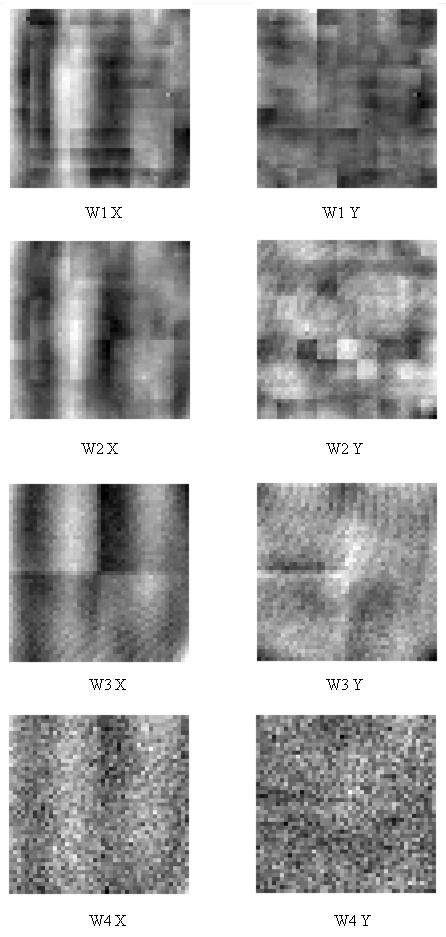 |
The residual structure is highly correlated across bands, and so the band-to-band alignment error is considerably smaller than the in-band residuals.
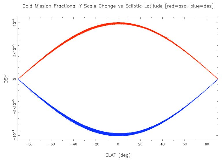
Differential aberration affects band-frame reconstruction via an apparent periodic change in plate scale. At its maximum near the ecliptic plane, the change is approximately 1 part in 10000, and the direction of that change reverses for ascending and descending scans. Figure 10 presents the theoretical model of the fractional change in Y plate scale as a function of ecliptic latitude for ascending (red) and descending (blue) scans. The X effects are essentially identical. The varying thickness of these lines reflects seasonal variations, with inner and outer envelopes near summer and winter solstices, respectively. If left uncorrected, this effect would contribute up to a maximum of 0.2 arcsec radial error for array-corner sources in the ecliptic observed near winter solstice. Theoretical corrections were made despite the fact that the effects are too small to threaten the astrometric requirements, because the other astrometric errors turned out to be small enough so that these effects were not washed out.
 |
The geometrical effects of differential aberration on array scale are made visible in the following exercise employing real survey data: two full distortion fits were generated using only frames within 20 degrees of the ecliptic from 25 days of the survey; one fit used only ascending scans, and the other used only descending scans. Then the descending-scan model was subtracted from the ascending-scan model. The difference between the two models is twice the distortion induced near the ecliptic by differential aberration alone. The vector-flow diagram for the difference is shown in Figure 11 with a scale factor of 250.
 |
Motion-induced aberration is a relativistic phenomenon that results from the speed of light not being infinite, i.e, motion of the observatory is generally not negligible compared to the motion of arriving photons. When the observatory's velocity vector is parallel to the look direction, the light is Doppler-shifted, and there is no aberration. When these directions are mutually perpendicular, there is no Doppler shift, and the aberration is maximal. For intermediate alignments, both Doppler shifting and aberration occur; we will be concerned only with the aberration herein. When the ratio of the observatory's velocity magnitude v to the speed of light c is very small, a simple non-relativistic formula provides a good approximation for the aberration shift. In the case of WISE, the observatory velocity relative to the ICRF system is the vector sum of the earth's velocity about the sun and the spacecraft's velocity about the earth. The magnitude of this ranges from about 22.3 to 37.4 km/s, so that v/c is on the order of 10-4, which allows the nonrelativistic formula to be used with an approximation error in differential aberration of less than 0.5 milli-arcsec over the WISE array.
The diagram in Figure 12 below shows a vector of arbitrary length L at an angle θo as measured in the rest frame, the XY coordinates. The telescope moves in the X direction with speed v. It takes light a time L/c to travel the distance L (which is going to cancel out below), and during this time, the telescope moves a distance vL/c, making the object appear to be at the angle θs.
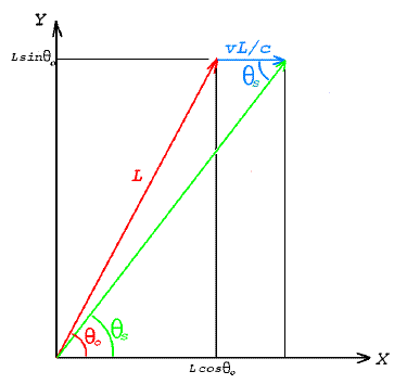 |
The tangent of θs is seen to be
 |
(Eq. 37) |
To get an expression for the shift itself, we define Δθ = θo - θs and use the law of sines to obtain
 |
(Eq. 38) |
Canceling L and rearranging,
 |
(Eq. 39) |
In our case, Δθ is small enough to ignore the distinction between Δθ and sinΔθ. Each WISE frame's FITS file contains the components of the spacecraft's total ICRF velocity vector in the header. This vector is transformed into the array's frame coordinates to obtain the components in that system, (Vfx,Vfy,Vfz). The last component is the one that causes Doppler shifting and is of no interest herein. The diagram in Figure 13 below shows the velocity vector V in frame coordinates and the shift Δθ in the plane formed by the velocity vector and the Z axis, with components ΔX and ΔY on the X and Y axes, respectively. These are the total aberration shifts of the Z axis. At other locations in the array, the aberration components are slightly different because of the slightly different angles between the velocity vector and the look direction of the pixels at those locations. The computation is similar, however; one must simply rotate coordinates to a system in which a given pixel's look direction is the Z axis, which we will denote Zp.
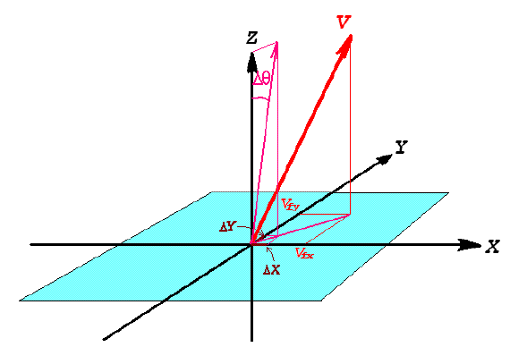 |
We compute ΔX and ΔY for any given Z axis by defining a unit vector U parallel to V and using it as follows.
 |
(Eq. 40) |
Denoting the aberration shifts of the center Z axis of the array as ΔX and ΔY, and denoting the shifts of a pixel's look direction Zp as ΔXp and ΔYp, the differential aberration at the pixel is
 |
(Eq. 41) |
In Figure 13 above, ΔX and ΔY are the frame coordinates where an object appears that would have appeared at (0,0) if the speed of light had been infinite. Therefore the look direction of the Z axis corresponds to the angle θo, not θs, whereas the latter is the angle that appears in Equation 39. If we wish to compute where a source will appear whose true position is known, Equation 39 provides that. But if we wish to correct the position of an object observed at ΔX and ΔY for aberration, in principle we would have to iterate Equation 39, starting with the solution for aberration at Z = Zp, subtracting that off to get a new Z, compute a better approximation of the aberration shifts to get a better approximation for Z, and continuing until the iteration converges. In practice, for WISE purposes, we do not iterate Equation 39 when correcting from observed to true position, since the maximum differential aberration shift is about 0.2 arcsec between the frame center and a corner that is about 10,000 times as far away from the center as this shift. Thus the differential aberration between a point in the array and another point less than 0.2 arcsec away is negligible, and we need not distinguish between θo and θs in Equation 39.
Since the WISE frame positions and orientations on the sky are reconstructed by matching WISE sources to astrometric references, there is no need to correct for total aberration. There is a residual effect, however, due to differential aberration that manifests as a time-dependent scale-factor change. Corrections for this effect are needed when calibrating optical distortion and when characterizing the total distortion in a WISE frame.
The offsets in Equation 41 are subtracted from WISE source positions used for calibrating optical distortion in order to remove the time-varying component of the total distortion (this correction is performed by the gndfab module). The resulting optical distortion coefficients are used in the scan-frame pipeline processing with frame-dependent corrections for differential aberration added to them. These corrections are in the form of SIP coefficients for a first-order distortion model. For a given frame, the spacecraft velocity vector is used by the diffabr8 module to compute the differential aberration on a uniformly spaced 31×31 grid of points spanning the array, and then these 961 samples are used to fit first-order polynomials defined by (compare to Equation 33, and see the table below it for notation)
 |
(Eq. 42) |
where the dA factors are the fit coefficients for the X axis, and the dB factors are the fit coefficients for the Y axis. Then during pipeline initialization the optical distortion SIP coefficients for the frame are modified according to
 |
(Eq. 43) |
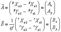
WISE tiles are constructed by mapping multiple frames from the scan/frame processing into a common coordinate system and co-adding them. The mapping of each frame depends on its scan/frame position reconstruction. The composite multi-frame image that constitutes a tile inherits varying degrees of position reconstruction error from its ingredient frames, and these may not average out to zero. The residual error was expected to be very small and turned out to be in practice, but the resources needed to correct the position bias and twist angle were very small, and so these adjustments were made to the tile image, and as a result, to the position of each point source extracted from the image. The correction on each axis and to the twist angle are recorded in the Atlas Metadata Table, so they can be removed if that is desired. No attempt to correct scale factor was made.
Assuming correct scale factors, the relationship between true and estimated tile position can be expressed in terms of offsets on each axis, ΔX and ΔY, and a rotation angle, θ. For example, given the coordinates of a source in the tile, (Xs,Ys), and correct coordinates (Xc,Yc), the relationship between the two is
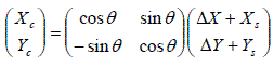 |
(Eq. 44) |
Tile position refinement is concerned only with adjusting tile positions relative to the astrometric standard used by WISE, the 2MRef sources, a subset of the 2MASS catalog. For this purpose, the subset we use is selected for low proper motions and good estimation quality:
We must also restrict the WISE sources to a subset designed for reliability. To this end we require the WISE sources to satisfy the following:
The WISE and 2MRef sources are matched in pairs by cross-correlating source lists with a match radius of 1 arcsec. This produces two lists containing the same number of sources, N, one from WISE and one from 2MRef, in one-to-one correspondence.
WISE source positions relative to each other are not modified, the entire tile is adjusted as a rigid body, affecting all source coordinates in the same way. The offsets and rotation above therefore correct only errors in the frame location and orientation. These corrections are expected to be very small (and this is what is found in practice). The diagram in Figure 14 below shows the geometry highly exaggerated for clarity.
 |
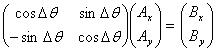
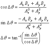
All source coordinates are in the U-scan system, mapped from their RA and Dec coordinates. The black (unrotated) axes constitute a 2MRef reference frame; its origin is the mean position of all the 2MRef sources, and the axes are aligned with U-scan for convenience. The blue (rotated and offset) axes are the WISE reference frame, whose origin is the mean position of all the WISE sources and is offset from the 2MRef system by ΔX and ΔY. The WISE and 2MRef sources are already paired. Except for the usual extraction errors, each has the same relationship to its own coordinate system, which implies that the two sets of axes are not perfectly aligned with each other. For example, the 2MRef source A has coordinates in its system that are ideally equal to those of the WISE source B in its respective system; if we subtract ΔX and ΔY from Bs U-scan coordinates, what remains is a vector that should have the same length as that of source A but is rotated relative to it in the U-scan system by the angle θ. Thus an appropriate rotation would bring the two sources into the same location. We can accomplish this offset subtraction by subtracting the U-scan coordinates of the 2MRef systems origin from all 2MRef U-scan coordinates and subtracting the U-scan coordinates of the WISE systems origin from all WISE U-scan coordinates. This eliminates ΔX and ΔY, leaving only the rotation as the difference between the two systems.
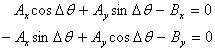
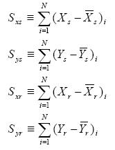
The rotation can be computed for each source pair. If there were no position errors due to the extraction process, any source pair would suffice, but since there are in fact such position errors, some averaging process is needed. We use a least-squares solution that minimizes the sum-squared radial distances between source pairs. Denoting this cost function R2, we have
 |
(Eq. 45) |
where the summation on i is over the N source pairs. Differentiating with respect to θ and setting to zero yields
 |
(Eq. 46) |
where
 |
(Eq. 47) |
This can be solved for θ to obtain
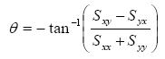 |
(Eq. 48) |
where
 |
(Eq. 49) |
We note in passing that except for 1/N normalization, these are just covariances. Since the WISE and 2MRef source coordinates are already very close, we can expect Sxx and Syy to be approximately equal to N times the sample variances of the X and Y coordinates respectively of either group, whereas we expect no correlation between X and Y coordinates, so Sxy and Syx should be relatively close to zero. As a result, the argument of the inverse tangent should be a very small number.
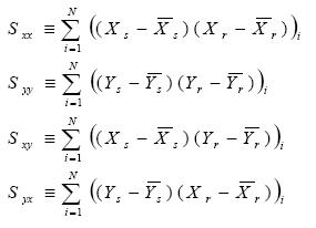
Since ΔX and ΔY are just the differences between the mean coordinates of the two groups, we have all three parameters of interest for correcting the positions of sources in the tile. Although the rotation angle is generally very small, technically we should account for the fact that ΔX and ΔY were defined in the 2MRef system, whereas we want to apply offset corrections to WISE sources in their own system, which requires rotating the offsets into that system:
 |
(Eq. 50) |
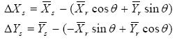
Each WISE sources coordinates are then corrected according to
 |
(Eq. 51) |
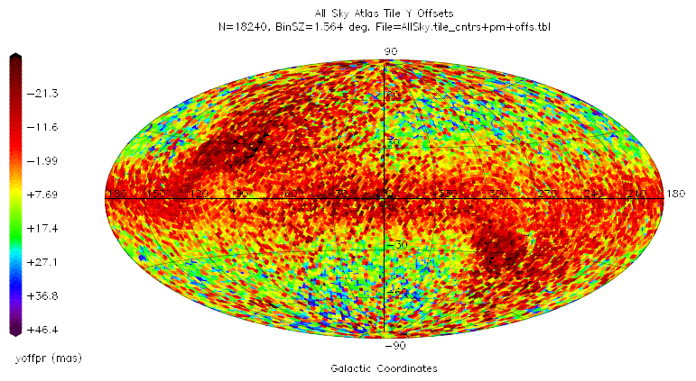
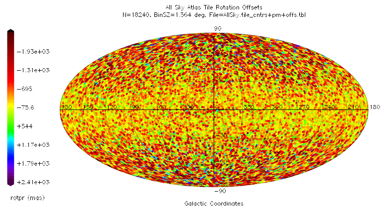
The average corrections over all of the 18240 atlas tiles are given in the table below.
| Correction | Mean | Standard Deviation |
| ΔXs | 1.4 mas | 17.3 mas |
| ΔYs | 7.5 mas | 15.6 mas |
| θ | 6.1 mas | 877.7 mas |
The following all-sky plots show the distribution of these corrections over the sky in galactic coordinates.
After-the-fact analyses of the alignments between the band-frame systems using large quantities of processed data indicate that the Y offset from W1 used for W3 was wrong by approximately 75 mas, and the Y offset for W4 was wrong by about the same amount. W2 looks good. The band-frame reconstructions were done tying W1 to 2MRef, and the other three bands were dragged along using a priori band-to-band knowledge. The magnitude of this error on merged source positions will depend on how heavily the longer wavelength bands are weighted. For four-band sources it will be relatively small, given the larger uncertainties associated with the longer wavelength bands. Sources seen only in W3 and/or W4, on the other hand, will feel the full effect.
The band-frame positions are reconstructed using a selected subset of 2MASS (2MRef) as the reference catalog. Given that 2MASS does not include proper motion information, there will be systematic differences between the WISE positions and corresponding positions measured independently in an of-date inertial reference system. These systematic differences can vary in magnitude and direction with sky position. This effect is discussed in VI.4.f).