
| AWAIC: A WISE Astronomical Image Co-adder | |
Below we summarize the WISE co-adder (image mosaicker). It can mosaic any number of images, avoiding "bad" and/or outlying input pixels masked a priori in the process. This software is part of the multi-frame processing subsystem of the WISE Science Data System (WSDS). Other related modules are "Bmatch" for background (offset) matching, and "AWOD" for temporal outlier detection and masking. These are normally executed prior to AWAIC.
Related documents, papers and presentations are as follows:
AWAIC is capable of resolution enhancement using an iterative (Richardson-Lucy like) procedure. However, this is not in the WSDS baseline design, and will not be performed in automated operations. The WISE Atlas image products (deliverables) will be simple co-adds based on a PRF-interpolation scheme. If desired, resolution-enhanced products will only be made offline. This is because much hands-on analysis and tuning is needed for optimal enhancement, e.g., in the construction of PRFs at different FPA locations and the removal of artifacts. Also, the iterative procedure itself is CPU intensive.
Very briefly, AWAIC is based on using the detector's Point Response Function (PRF) as an interpolation kernel when re-projecting and re-estimating pixels in an upsampled mosaic grid. Conventional image co-adders like IPAC's MONTAGE and MOPEX tools are based on simple overlap-area-weighted averaging. In fact, PRF-interpolation or "PRF-weighted" averaging implicitly reduces to an area-weighted method when a detector's PRF is approximated by a top-hat (flat) function spanning ~ 1 detector pixel. This is also true if the telescope's optical Point Spread Function (PSF) is undersampled by a detector. In this case, the PRF is close to top-hat anyway and area-weighted interpolation/averaging is the only way to proceed.
So, why use the PRF as an interpolation kernel? There are two reasons: The first is that the detector's PRF represents the actual real transfer function from which sky flux ("the truth") propagates through the measurement process to yield the observations. Other mock interpolation kernels (overlap-area weighting, sinc etc..) are mere approximations. These usually yield simple (and esthetic) co-adds, but don't make use of the full spatial information collected by a detector's pixel if it happens to oversample the optical PSF of a telescope. The second reason is that use of a PRF kernel directly allows for resolution enhancement if one decides to deconvolve its effects from the data (e.g., through a Richardson-Lucy process). Even if one has a detector which undersamples the PSF, one can still gain spatial resolution using iterative methods if multiple overlapping (randomly dithered) observations are available. The random dithering, in effect, reconstructs the PRF.
The method used in AWAIC is similar to that used by the 2MASS co-adder. The main difference is that the 2MASS co-adder assumed an analytic function for its interpolation kernel, derived by assuming a 2D Gaussian for the PSF (seeing profile) convolved with the square pixel response. This function was optimized such that "shape-bias" from "square" detector pixels was minimized (smoothed out), but not so much that excessive variance was introduced from over-smoothing. Also, since the seeing PSF was undersampled by the 2MASS detectors, the assumed interpolation kernel played more the role of a "smoothing kernel", e.g., for reducing pixel-shape bias. The direct use of a measured PRF as the interpolation/smoothing kernel in 2MASS co-addition was not possible due to the unstable and stochastic nature of the seeing. It's important to note that AWAIC can also mimic the 2MASS method in that it allows any interpolation kernel to be specified, whether it be the actual PRF, or, an analytic function fit.
We now outline the basic algorithm for simple image co-addition and optional resolution enhancement as implemented in AWAIC. The algorithm is based on the Maximum Correlation Method (MCM), as previously implemented in IPAC's HIRES tool. AWAIC includes generic functionality to handle images in standard FITS format, omit masked input pixels, allow non-isoplanatic PRFs, include prior noise-variance weighting, and suppress ringing artifacts from the resolution enhancement.
MCM essentially incorporates classic Richardson-Lucy, but first and foremost, it is an image-reconstruction algorithm. It was first (and still) used to generate FRESCO image products from IRAS data. MCM's goal is to build a model of the sky (truth) which reproduces, and is "maximally consisent" with the observations via transfer by the PRF. The main steps of the MCM are as follows.
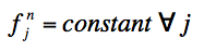
(1). First, we begin by assuming a flat, nonzero model of the sky (the model co-add image):
 |
(Eq. 1) |
(2). Next, we use the detector PRF(s) to "observe" this model (flat) image. We predict the observed flux, Fi, in each detector pixel i from the model image by convolving it with the characteristic PRF centered at each detector pixel:
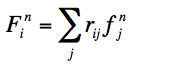 |
(Eq. 2) |
(3). Correction factors are computed for each detector pixel i by dividing their observed flux, Di, by that predicted from the model (Eq. 2):
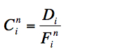 |
(Eq. 3) |
(4). For each pixel j in the model co-add, all "contributing" correction factors (i.e., contributed by the overlapping PRFs rij of all neighboring detector pixels i) are averaged using response-weighted averaging:
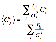 |
(Eq. 4) |
(5). Finally, the original (or starting) model image pixels are multiplied by their respective averaged correction factors (Eq. 4) to obtain new estimates of co-add model fluxes:
 |
(Eq. 5) |
If we are simply after a PRF-interpolated co-add/mosaic, we terminate the process here. The final co-add pixel fluxes are then given by fjn=2, where we started with a flat model image: fjn=1 = constant (Eq. 1).
If we desire resolution enhancement, the process is iterated by using the new and "better" model sky from Eq. 5 as input into Eq. 2. Thus, the model is continuously "re-observed" with the detector-PRFs to keep on producing a better model sky (Eq. 5). With patience, this eventually becomes the final co-add image with resolution that may exceed the diffraction limit of the optical system. The iteration stops when either the difference between the model pixel correction factors from successive iterations: |Cjn - Cjn-1| becomes tiny (below some threshold), and/or the Cjn values themselves are close to unity. When this is satisfied, the process has converged and the sky flux is said to have been resolved to an extent determined by the accuracy of the PRFs. So, subjecting a simple model image to the above simulation and feedback correction process "decorrelates" the model pixels. It is an algorithmic property of MCM that this decorrelation modifies the starting (flat) model image only to the extent necessary to make it reproduce the measurements to within the noise.
It's important to keep in mind that the very first iteration of MCM (which starts with a flat model at Eq. 1 and terminates at Eq. 5) yields the PRF-interpolated co-add/mosaic. This will be the default for all WISE Atlas image products. Further iterations imply resolution enhancement.
Accompanying the primary co-add intensity image, AWAIC also generates a depth-of-coverage map and an uncertainty image. The depth-of-coverage map is an image of the same size as the co-add. This effectively indicates how many times a point on the sky was visited by a "good" detector (FPA) pixel, i.e., not rejected due to prior-masking, cosmic rays or other transients. The depth-of-coverage at a co-add pixel j is given by the sum of all overlapping (unit volume-normalized) PRF contributions at that location:
 |
(Eq. 6) |
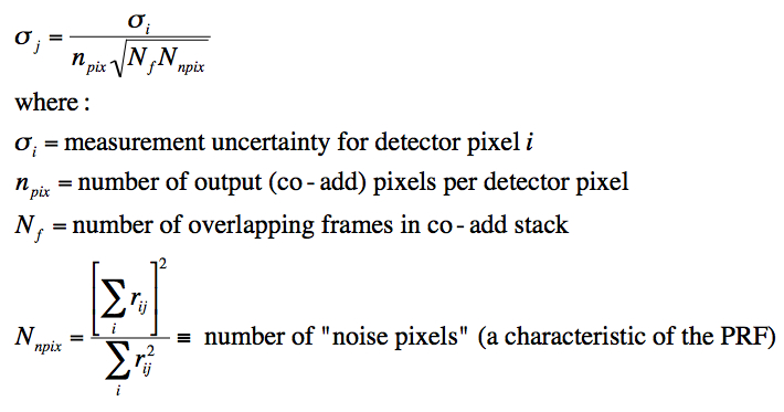
The uncertainty image will contain a 1-sigma error estimate in the co-added signal at every pixel. Given an uncertainty σi for an input detector pixel i, the uncertainty in the response-weighted average (Eq. 4) at co-add pixel j is given by:
 |
(Eq. 7) |
For full algorithmic details, noise properties and methods for source photometry on AWAIC co-adds, see the Software Design Specification (SDS) document.
AWAIC is written in ANSI/ISO C. A synopsis and command-line usage of the program is below.
Usage: awaic
 -f1 <inp_image_list_fname>  (Required; list of images in FITS format)
 -f2 <inp_mask_list_fname>   (Optional; list of bad-pixel masks in 32-bit INT
                              FITS format; only values 0 -> 2^31 are used)
 -f3 <inp_uncert_list_fname> (Optional; list of uncertainty images in
                              FITS format)
 -f4 <inp_prf_list_fname>    (Required; list of PRF FITS images each
                              labeled with location on array)
 -f5 <inp_mcm_mod_image>     (Optional; input starting model image to
                              support MCM; Default = flat image of 1's)
 -m  <inp_fatalmask_bits>    (Optional; bitstring template specifying
                              pixels to flag as set in input masks; Default=0)
 -X  <mosaic_size_x>         (Required [deg]; E-W mosaic dimension
                              for crota2=0)
 -Y  <mosaic_size_y>         (Required [deg]; N-S mosaic dimension
                              for crota2=0)
 -R  <RA_center>             (Required [deg]; RA of mosaic center)
 -D  <Dec_center>            (Required [deg]; Dec. of mosaic center)
 -C  <mosaic_rotation>       (Optional [deg]; in terms of crota2:
                              +Y axis W of N; Default=0)
 -ps <pixelscale_factor>     (Optional; output mosaic linear pixel scale
                              relative to input pixel scale; Default=0.5)
 -pa <pixelscale_absolute>   (Optional [asec]; output mosaic pixel scale
                              in absolute units; if specified, over-rides -ps)
 -pc <mos_cellsize_factor>   (Optional; for PRF placement: internal linear
                              cell pixel size relative to mosaic pixel size;
                              =input PRF pixel sizes (-f4); Default=0.5)
 -sf <pixelflux_scale_flag>  (Optional; scale output pixel flux with pixel
                              size: 1=yes, 0=no; Default=0)
 -sc <simple_coadd_flag>     (Optional; create simple co-add/mosaic using exact
                              overlap-area weighting: 1=yes, 0=no; Default=0)
 -n  <num_mcm_iterations>    (Optional; number of MCM iterations;
                              Default=1 => coadd, no resolution enhancement)
 -rf <rotate_prf_proj_flag>  (Optional; rotate PRF when projecting input
                              frame pixels: 1=yes, 0=no; recommended for -n > 1
                              if PRF severely non-axisymmetric; Default=0)
 -ct <prf_cell_size_tol>     (Optional [asec]; maximum tolerance for difference
                              between cell-grid pixel size [-pc] and input
                              PRF pixel size; Default=0.0001 arcsec)
 -if <interpolation_option>  (Optional; method for interpolating PRF onto
                              co-add cell-grid: 0=nearest neighbor,
                              1=area-overlap weighting [only possible for
                              -n = 1 & -rf = 0]; Default=0)
 -o1 <out_mosaic_image>      (Required; output mosaic image FITS filename)
 -o2 <out_mosaic_cov_map>    (Required; output mosaic coverage map FITS
                              filename)
 -o3 <out_uncert_mosaic>     (Optional; output uncertainty mosaic FITS
                              filename; only applicable to -n = 1 co-adds;
                              based on input prior uncertainties)
 -o4 <out_stddev_mosaic>     (Optional; output standard deviation mosaic
                              FITS filename; only possible under -sc 1)
 -o5 <out_corfac_mosaic>     (Optional; output mosaic of MCM
                              correction-factors; only valid when -n > 1)
 -o6 <out_cfvuncert_mosaic>  (Optional; output mosaic of data derived
                              MCM uncertainties (from CFV); only valid
                              when -n > 1)
 -o7 <out_cellmosaic_image>  (Optional; output mosaic basename in upsampled
                              cell-grid frame; for debug or resuming MCM later;
                              will be appended with mcm iteration number)
 -o8 <out_cellcfv_image>     (Optional; output CFV mosaic basename in upsampled
                              cell-grid frame for debug purposes; will be
                              appended with mcm iteration number)
 -g                          (Optional; switch to print debug statements
                              to stdout and files)
 -v                          (Optional; switch to print more verbose output)
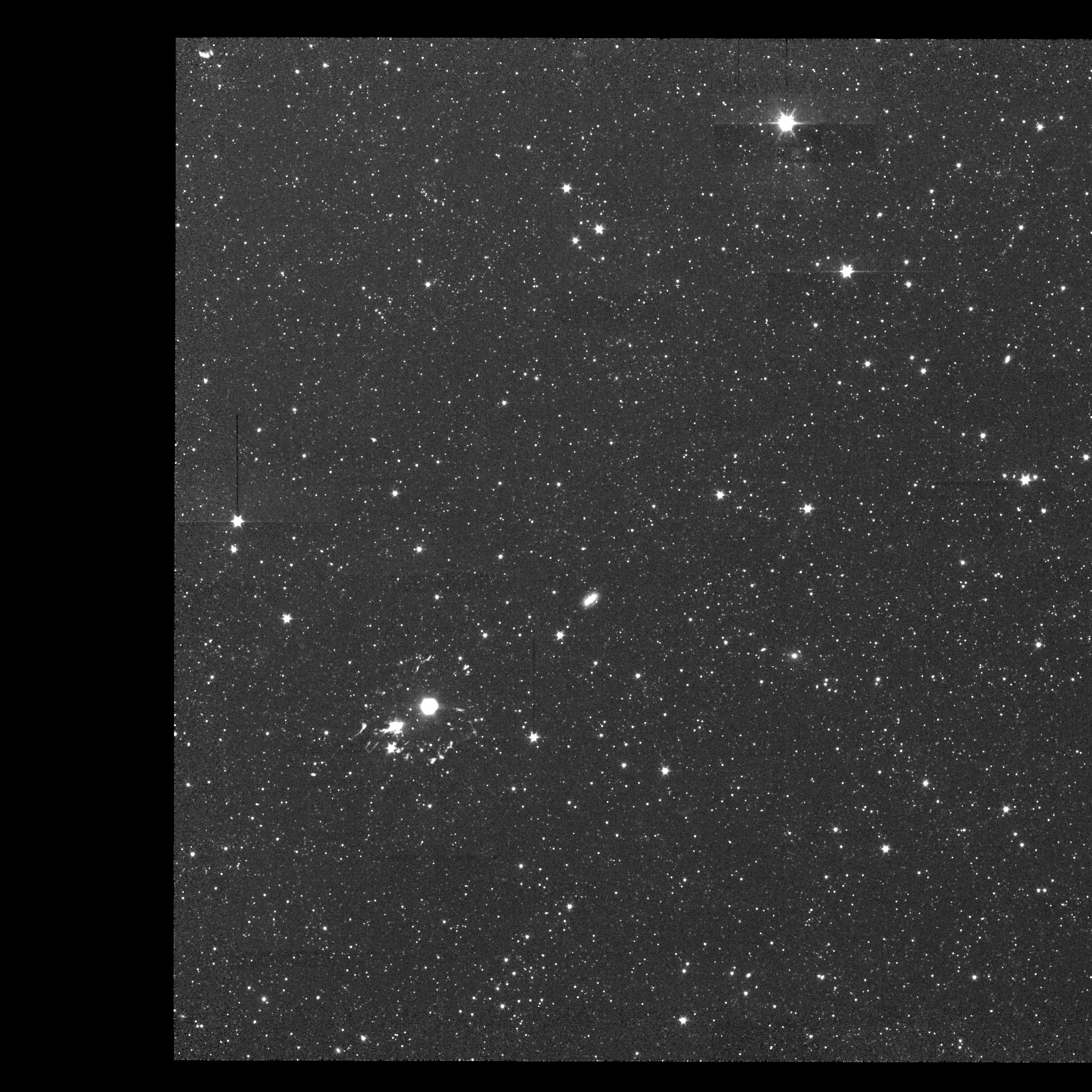
We simulated a 1.4° × 1.4° region of sky containing exclusively point sources, then cut-out eight interleaved image frames each matching the WISE FOV (~47′ × 47′, or, 10242 pixels at 2.75″/pixel). The frames were then convolved with a realistic band-1 WISE PRF. Single spike radiation hits and Poisson noise were then added. "Bad" pixels were assumed and flagged in masks corresponding to each image frame. The simulated radiation-hits were also flagged and recorded in these masks. All masked pixels were omitted from the AWAIC co-adds.
The series of figures below shows a snippet of the simulation
region with various co-adds/mosaics reconstructed from the frame images
using AWAIC. A comparison with the
MONTAGE tool is also shown.
 |
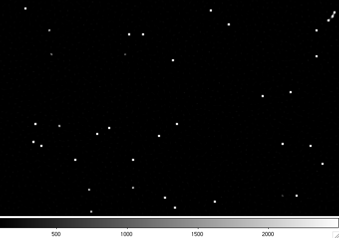
| Figure 1 - "Truth" image of simulated region containing point-source spikes. |
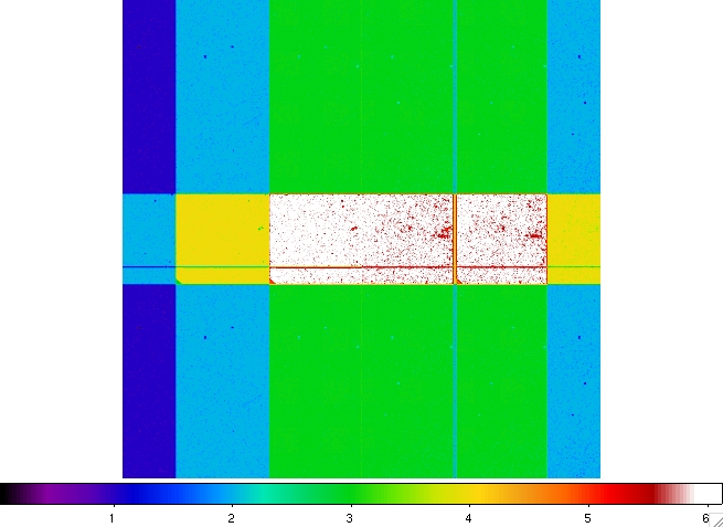 |
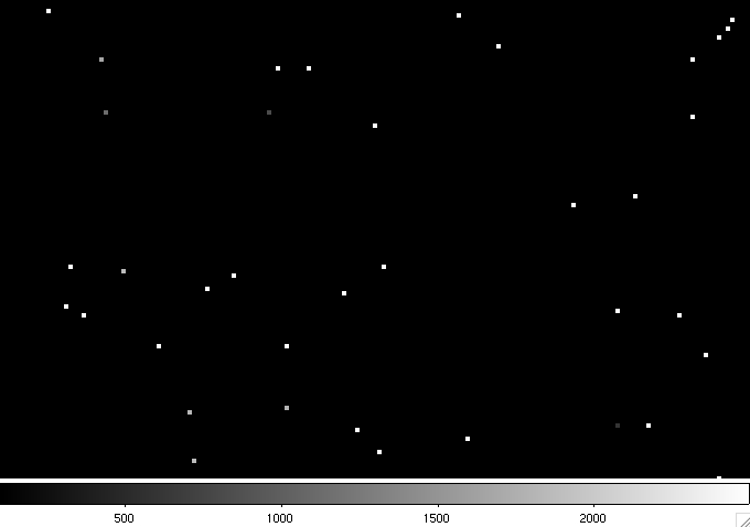
| Figure 2 - Depth-of-coverage map of the full simulated region from AWAIC. The range is 1 frame (blue) to 6 frames (white). Note: the spots are due to masked (missing) pixels, i.e., mock "bad" pixels and simulated radiation hits that were omitted from the co-adds below. The vertical and horizontal lines are due to masked pixels around the border of each frame - the so called "reference-pixels" surrounding the active region of each WISE frame. |
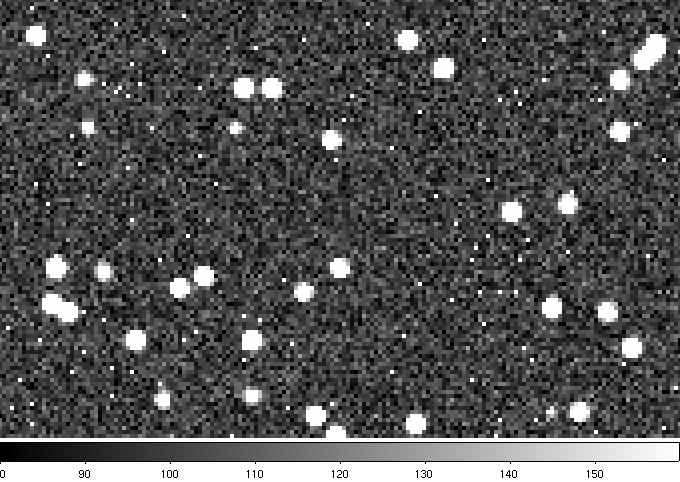 |
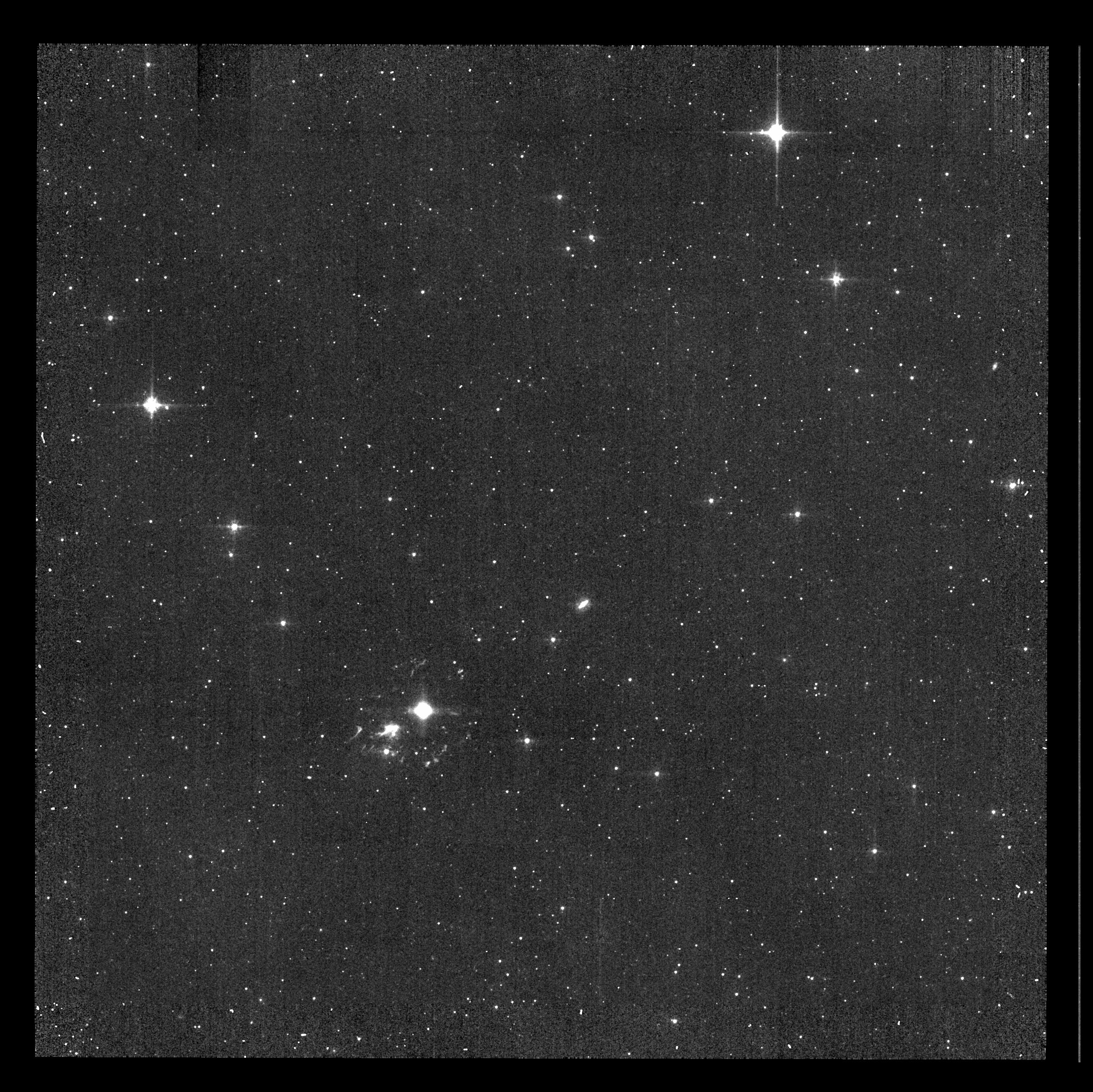
| Figure 3 - Same region in one of the "raw" image-frame cutouts after convolving with a PRF, and adding radiation hits and noise. |
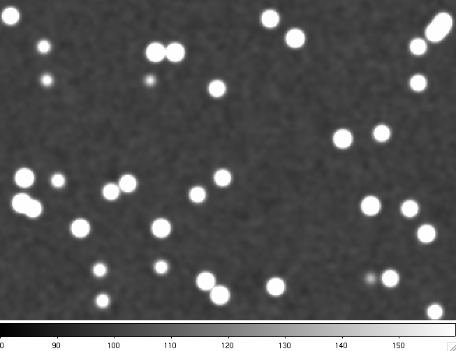 |
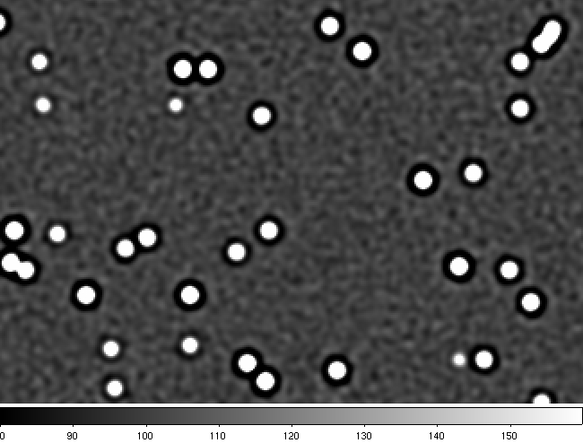
| Figure 4 - Co-add from AWAIC after n = 1 iteration (≡ simple PRF-interpolated co-add). Bad pixels and radiation-hits have been masked and omitted from the co-add. It's important to note that AWAIC has a tendency to smear structure right down to the pixel scale. Any missed radiation-hits and/or hot pixels will masquerade as point sources in the co-add. Thus, it is crucial that they are found and masked prior to co-addition. |
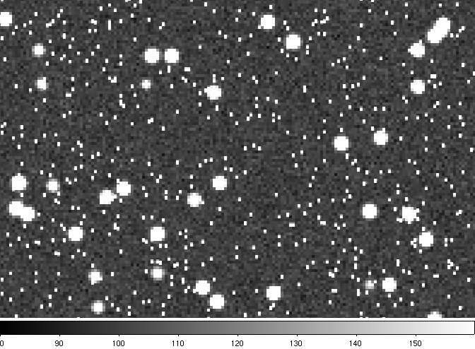 |
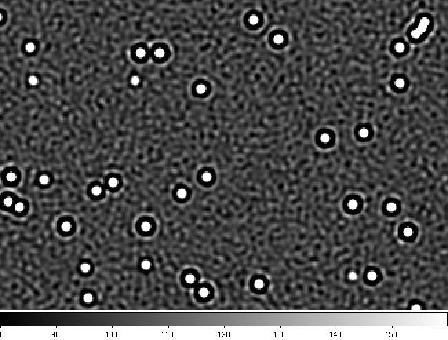
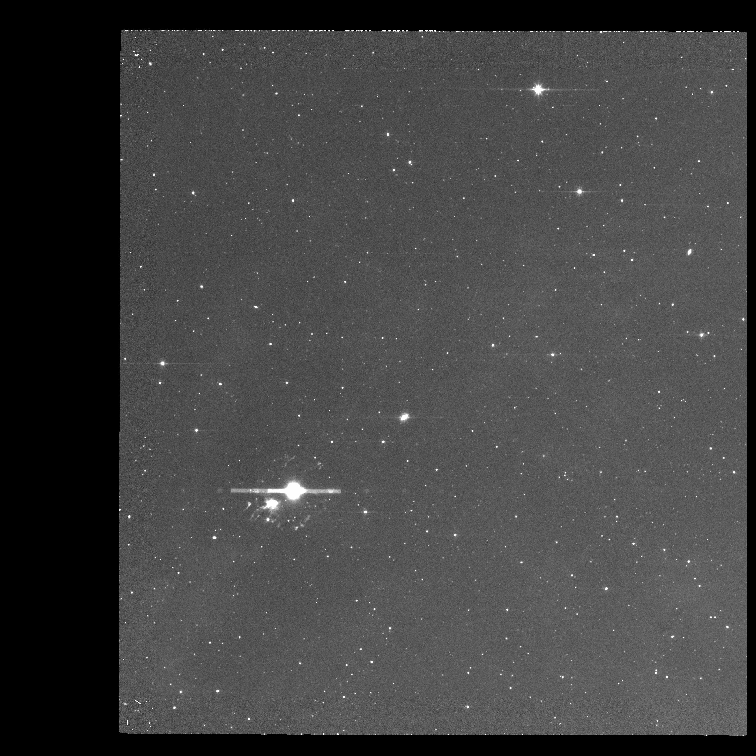
| Figure 5 - Co-add of same region using MONTAGE. Compared to AWAIC (Fig. 4), the sources are not as smooth since the MONTAGE method is effectively interpolation with a top-hat PRF (≡ area-weighted averaging). This leads to pronounced pixelization. Also, the MONTAGE software does not have the ability to mask bad pixels and radiation hits. The single-pixel spikes seen here are unfiltered radiation hits. |
 |
| Figure 6 - Co-add from AWAIC after n = 5 iterations. Note the inevitable "ringing" artifacts. |
 |
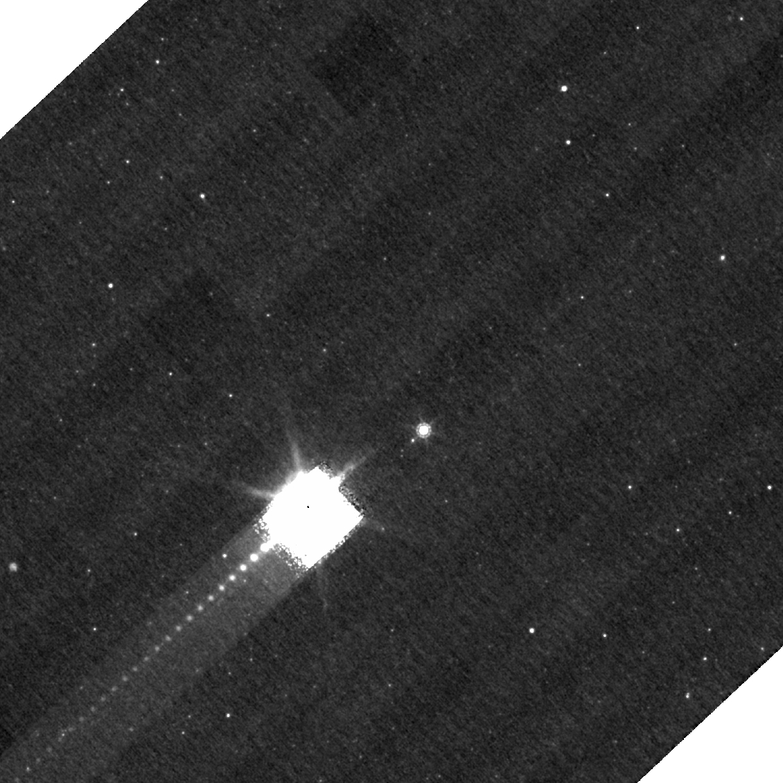
| Figure 7 - Co-add from AWAIC after n = 30 iterations. The point sources are sharper and more resolved compared to Figs 4 and 6. Much of the energy however (~several percent) goes into "ringing", but, see Fig. 8. |
 |
| Figure 8 - Co-add from AWAIC after n = 100 iterations with "ringing suppression" turned on. This involves removing the background from each input frame except for a tiny positive residual (of order ~1E-15%) prior to co-addition. This prevents sources to "ring" against the background level and their flux is forced to go where it belongs - the sources themselves. The stretch has been set to enable comparison with Fig. 1 - the truth image. As seen, the "truth" is just about reconstructed! |
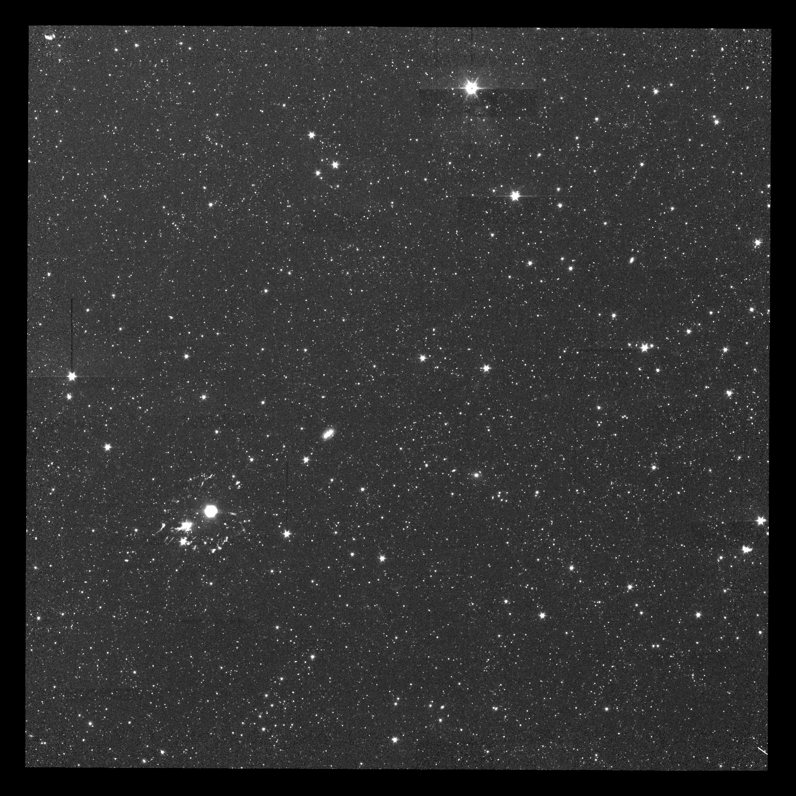
We experimented on a 3.6μm IRAC map of NGC 2403. A single PRF from the IRAC-Data Analysis website was assumed for the AWAIC co-add. Note: this PRF was not adequate for optimal resolution enhancement. The best PRFs to use are those derived directly from the image data, and at different array locations if possible.
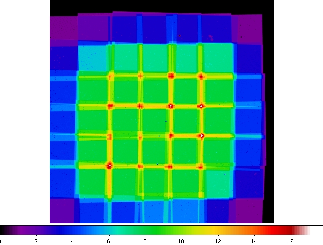 |
| Figure 9 - Depth-of-coverage map of the imaged region from AWAIC. The range is 1 frame (purple) to ~16 frames (red). Note: the spots are due to masked (missing) pixels. |
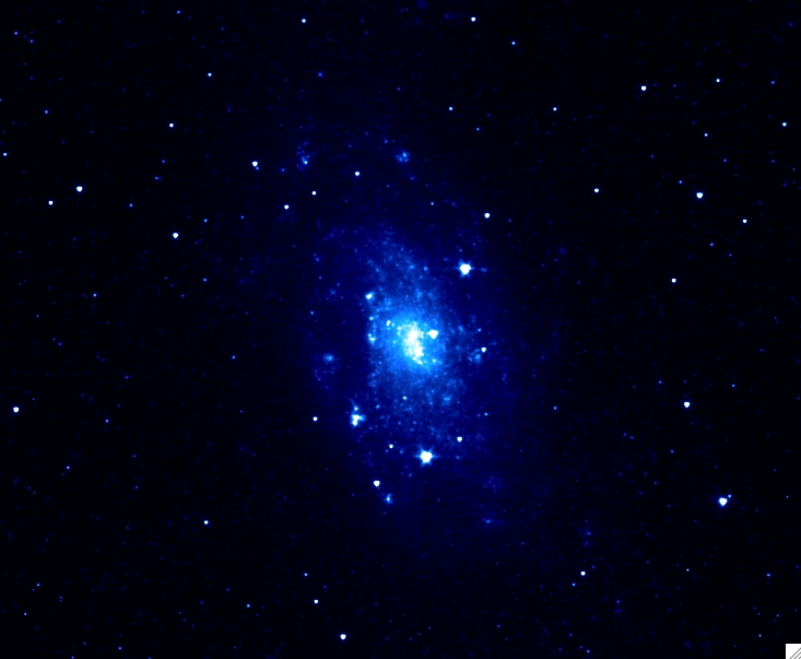 |
| Figure 10 - NGC 2403: co-add from AWAIC after 1 iteration (≡ simple PRF-interpolated co-add). For comparison, the co-add made with MONTAGE can be found here. At the time of writing, MONTAGE did not have the ability to omit prior-masked pixels, hence the peppered appearance. Click on panel to enlarge. |
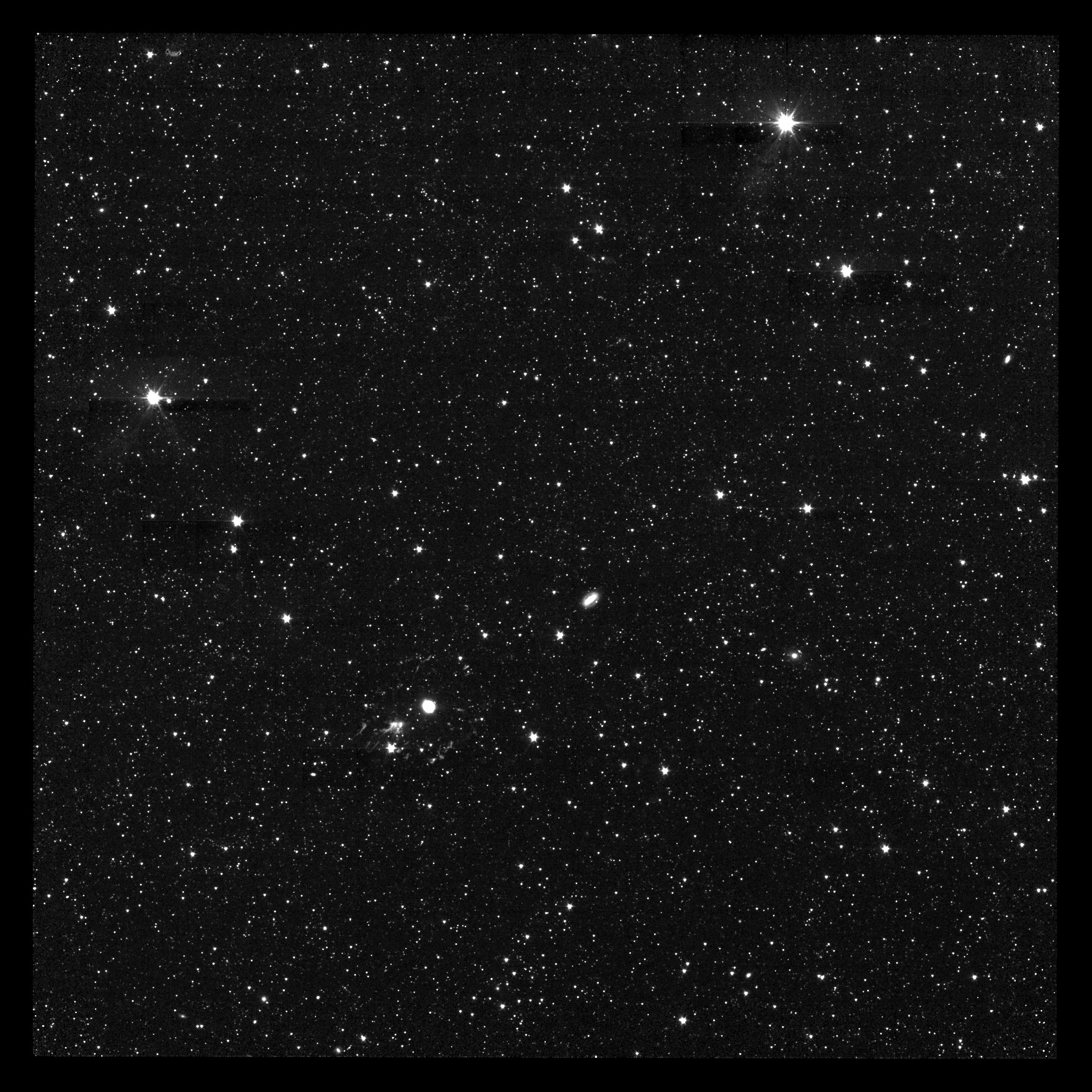
The following links show mosaics of the NEP made from IRAC observations at 3.6μm, 4.5μm, 5.8μm, 8μm (bands 1 - 4), and MIPS-24μm (band 1) taken in mid August 2007 (epoch 1 observations). This represents a region ~50 x 50 arcmin2 that will be observed by WISE on nearly every orbit. It is also called the "WISE Touchstone Field".
Here are the IRAC mosaics generated using AWAIC but with outliers first
detected by the
MOPEX
software and masked prior to co-addition:
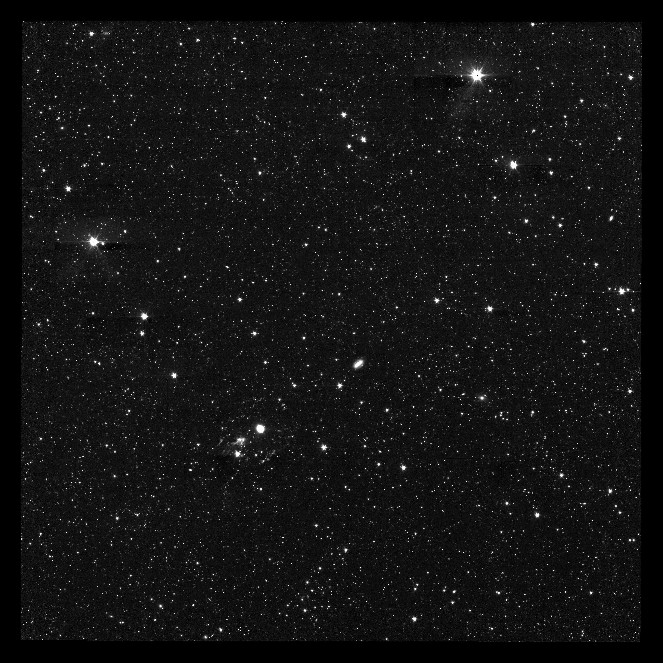
- AWAIC: NEP_IRAC_band1
- AWAIC: NEP_IRAC_band2
- AWAIC: NEP_IRAC_band3
- AWAIC: NEP_IRAC_band4
Here's the MIPS-24μm mosaic:
- AWAIC: NEP_MIPS_band1
And here's the corresponding depth-of-coverage map:
- AWAIC: NEP_MIPSband1_coverage_map
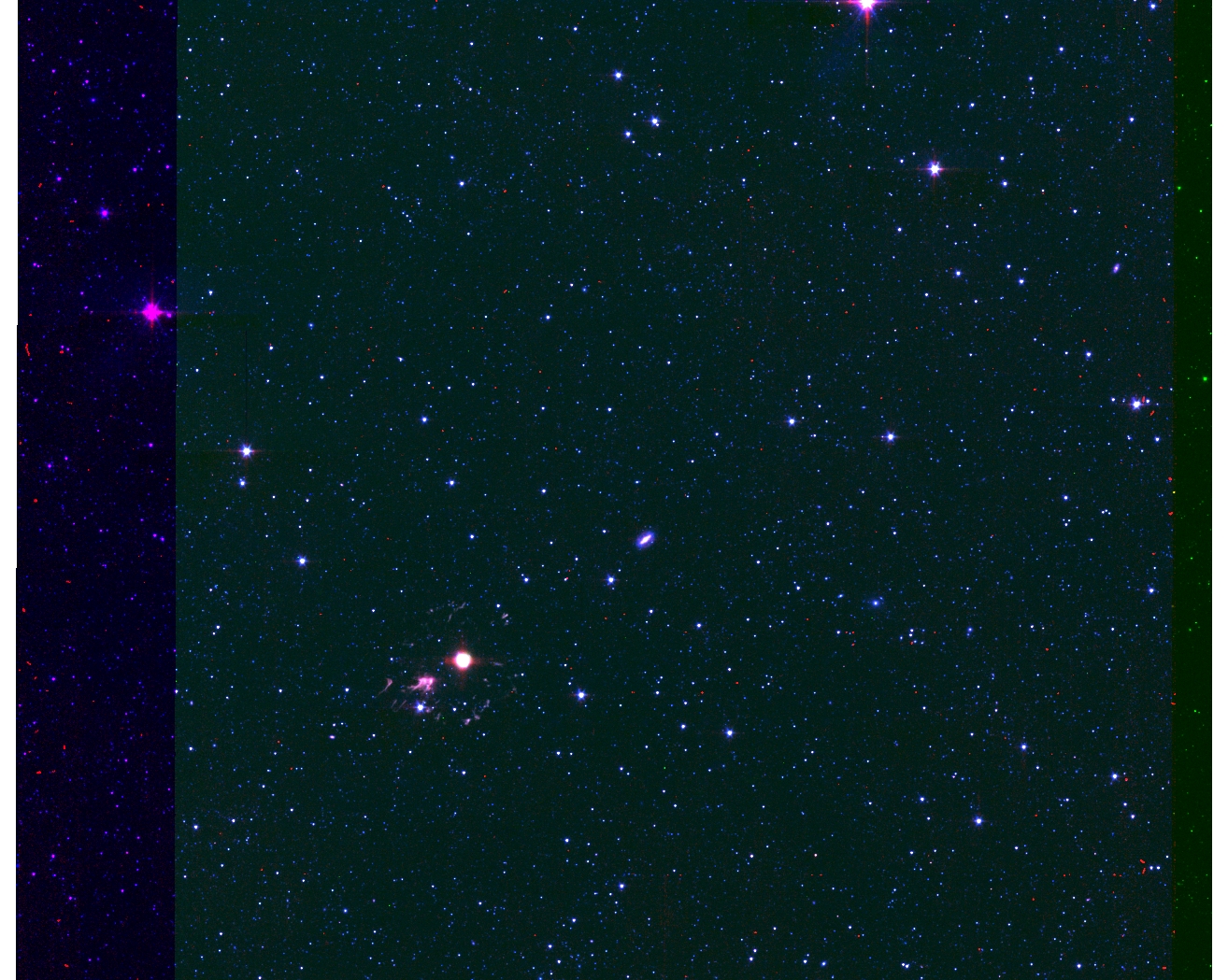
Here's a multi-color mosaic of a central portion that combines IRAC bands 1 (blue), 2 (green) and 3 (red):
- AWAIC: NEP_IRAC_bands1+2+3
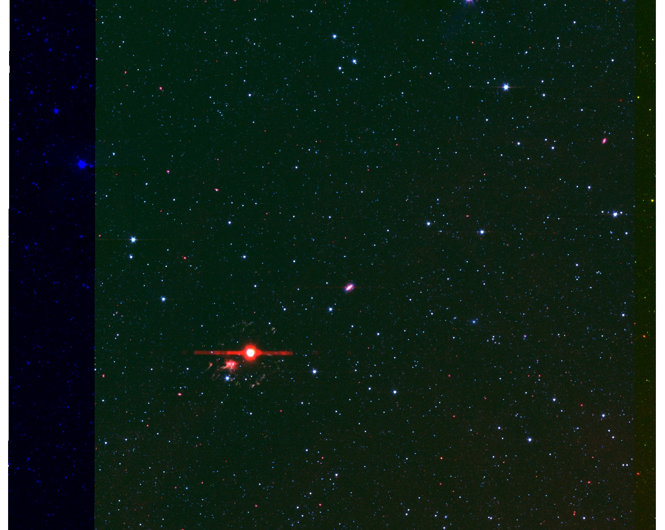
Here's a multi-color mosaic of a central portion that combines IRAC bands 1 (blue), 2 (green) and 4 (red):
- AWAIC: NEP_IRAC_bands1+2+4
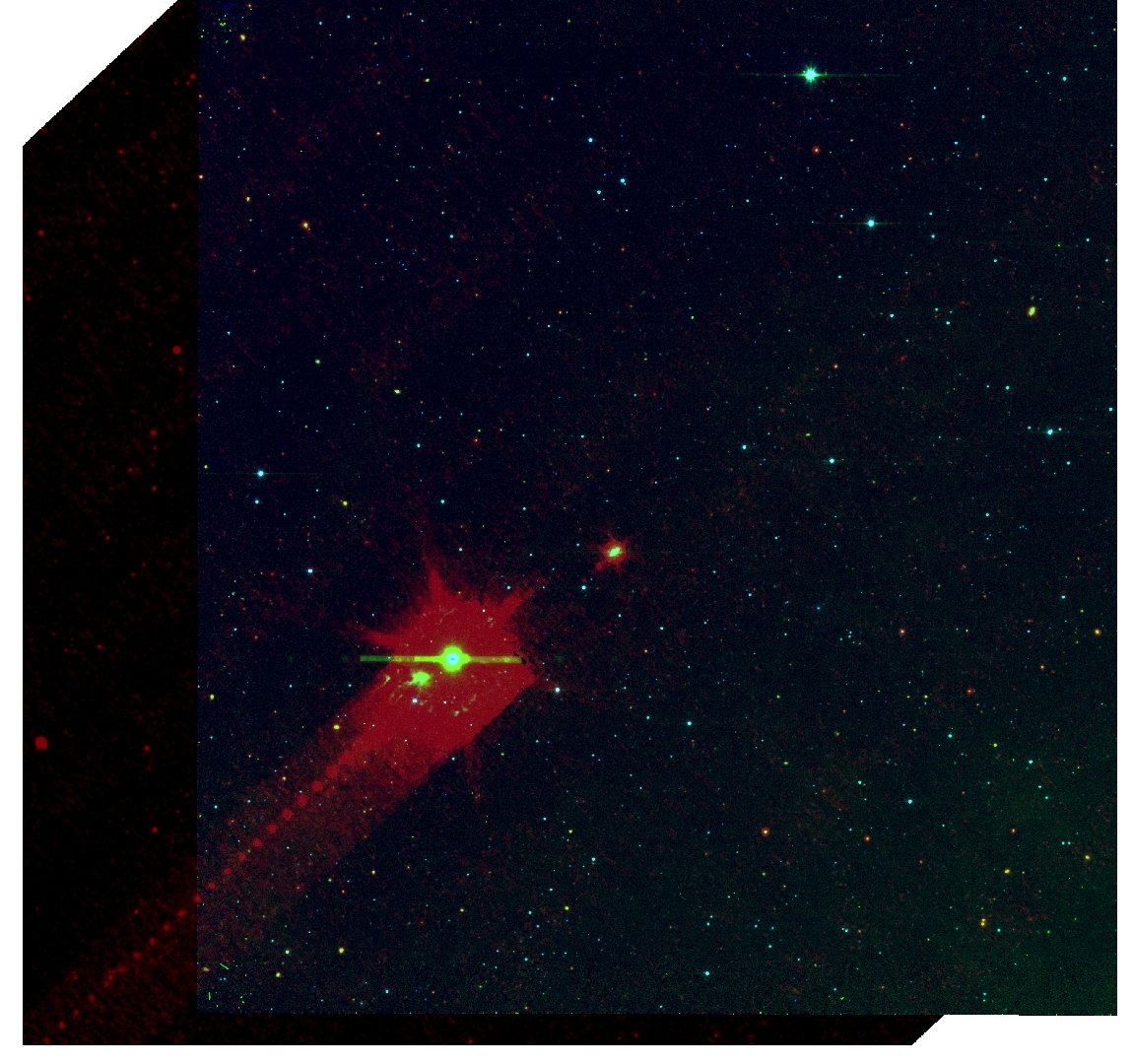
Here's a multi-color mosaic that combines IRAC bands 2 (blue), 4 (green) and MIPS-24μm (red):
- AWAIC: NEP_IRACbands2+4+MIPSband1
For comparison, here are the mosaics generated using MOPEX:
- MOPEX: NEP_IRAC_band1
- MOPEX: NEP_IRAC_band2
- MOPEX: NEP_IRAC_band3
- MOPEX: NEP_IRAC_band4
- MOPEX: NEP_MIPS_band1
Mosaics made from Spitzer and 2MASS observations of the SEP can be found here. These mosaics exercised the full suite of coaddition modules planned for WISE: Bmatch for background (offset) matching, and AWOD for temporal outlier detection and masking. These were executed prior to AWAIC.
Here we address the question: is the integrated flux within some aperture placed
on an input frame consistent (within measurement error) with that
measured at the same WCS location in a mosaic? We have explored this
statistically using the IRAC band-1 NEP case from section IV.3.1 above.
We placed an aperture
of radius ~18 arcsec (~15 native frame pixels) in each of the input frames,
summed the flux from all pixels, then placed the same size aperture
at the corresponding world coordinates in the mosaic and also summed the flux.
Results for the difference (frame - mosaic) and ratio (frame/mosaic) of
the integrated fluxes are shown in Figures 4a/b.
Our null hypothesis is that the mean difference in fluxes is zero, or,
that the mean ratio is unity,
i.e., we want no bias to exist when all
random statistical fluctuations in frame and mosaic flux measurements
are considered.
We first outline some of the caveats in performing this test:
Figure 4a shows that a small (but statistically significant)
bias exists in the mean "frame - mosaic"
flux difference in the sense that frame aperture fluxes are larger
by ~1.5% on average. Note, we are ignoring here the "excess" with differences
>~ 7 since these correspond to frame aperture fluxes contaminated by hot pixels
and rad-hits (i.e., item 1 above). Overall, the 1-2% bias is
consistent with flux smearing in the mosaic (item 5 above).
A nice example of the effects of masking and omitting pixels from
co-addition with AWAIC can be seen what happens to the cores of bright
stars which have been masked due to saturation.
If one has good sampling of the PSF, then the PRF tails of
"good" neighboring pixels will tend to fill in the holes where
pixels are masked. This means that flux can still be recovered from
the sky at the location of masked pixels. In the end, the better
the sampling (e.g., much above Nyquist), the smaller the impact from
masked pixels.
Figure 13 represents cutouts of a bright star located at top right in the
IRAC band-1 NEP mosaics of section IV.3.1. The MOPEX co-adder
with its area-weighted
interpolation scheme simply replaces masked pixels by NaNs.
The AWAIC co-adder with its PRF-interpolation scheme uses all the
spatial information collected by the detector pixels,
i.e., their "sphere of influence" is larger.
Figure 14 shows profile cuts across pixel rows going through the core
of the star.
While the MOPEX case has missing flux at the core, a large fraction (>70%) is
recovered in the AWAIC case.
In the AWAIC mosaic however, the core is not completely desaturated.
This can be seen in Figs 13 and 14 where a
pixel remains depressed by ~20% relative to surrounding pixel values.
This is primarily due to the IRAC channel-1 data being undersampled and thus,
the PRF tails
of "good" neighboring pixels do not reach far enough into the
masked regions.
However, their long tails (truncated at ~5σ) do a pretty
good job at recovering flux. Better flux recovery can be achieved if
one has more frame dithers,
and/or performs resolution enhancement with an accurate PRF.
More on this later.
These observations have a detector coverage-depth of 4 (with no masking),
but after masking the AWAIC co-add achieves an effective
coverage of ~2.7 at the core of this star.
The coverage-depth from MOPEX is zero.
In conclusion, the impact of bad pixels can be
ameliorated if one makes use of all the spatial information
that can be collected by a pixel, and this is represented by its PRF.
The examples below use data from the Spitzer
MIPS-24μm detector to test the HiRes capability of AWAIC.
We used this band primarily because the PSF is better than critically
sampled (~1.2x better than Nyquist) and the gain from resolution
enhancement is most dramatic, even at low depth-of-coverage.
A ringing suppression algorithm was used on all cases.
The following links display movies of the resolution enhancement process
on M51 over 40 iterations, i.e., going from simple co-add
to HiRes image in Figure 18. The two movies correspond
to cases with and without prior outlier masking. For a description of the
Correction Factor Variance (CFV), see the caption to Figure 19. Please
be patient. Wait for them to load first.
Movie 1: no outlier rejection
Movie 2: with outlier rejection
This section uses AWAIC to explore the following:
We have addressed these issues by simulating 1000 randomly dithered,
overlapping image frames. All dithers were made to overlap within a central
region of a co-add grid spanning ~600x600 pixels at 1.375 arcsec/pixel.
Before making the random frame cutouts, a constant background of 1000 counts
per pixel was assumed. To assist in our aperture photometry analysis,
we also added a single "truth" point source of 500 counts at the center
of the co-add grid. We then convolved with a
Gaussian kernel with sigma=2.75 arcsec (=one input frame pixel)
truncated at 3-sigma. Pure Poisson noise was added to each frame cutout
by sampling from a Normal distribution with
variance equal to the pixel (mean) value.
In the end, all simulated frames have a background of 1000 modulo
Poisson noise. Sets of 1, 2, 4, 8, 16, 32, 64, 128, 256 and 512 frames
were then collected and co-added with AWAIC to make 10 separate co-adds.
Note:
Below we summarize the main results of this analysis.
Full details and derivations of the equations that appear in the following
sections are presented in the
Software Design Specification
(SDS) document.
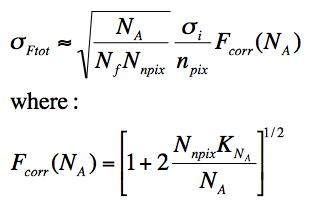
For a constant background level, constant
Poisson noise derived therefrom, and an isoplanatic PRF,
it is straightforward to show from Eq. 7 that the uncertainty
in a single co-add pixel j reduces to:
We performed aperture photometry on our simulated point source in all
10 co-adds. Three of these co-adds with overlayed apertures
are shown in Fig. 16. We assumed an aperture radius of 10 co-add pixels
throughout. This corresponds to ~2FWMH of the PRF. The background
annuli were chosen to have approximately the same number of pixels as the
source aperture.
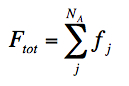
The total count in an aperture containing NA
pixels is the sum of all pixel counts:
The correction factor Fcorr(NA)
depends only on the PRF properties and the number of pixels in an
aperture, NA. This factor can be computed numerically
for different detector PRFs and a range of aperture sizes. A user
performing aperture photometry can then look up the appropriate value to apply.
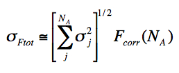
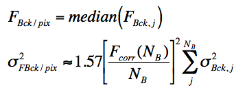
For a more accurate measure of the uncertainty in total counts in an
aperture when one has non-isoplanatic PRFs, a non-uniform background,
or, when there is much
variation in pixel values (and Poisson noise) as one always has
with a real source, the following expression is
more appropriate:
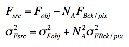
In general, the equations for source flux Fsrc
and its variance from aperture photometry can be written:
One can estimate the background per pixel in an annulus containing
NB pixels using either the mean:
4. Flux Conservation Check
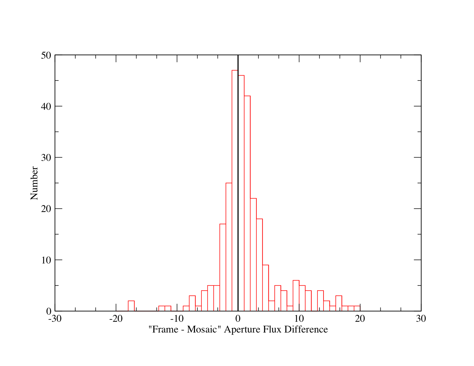
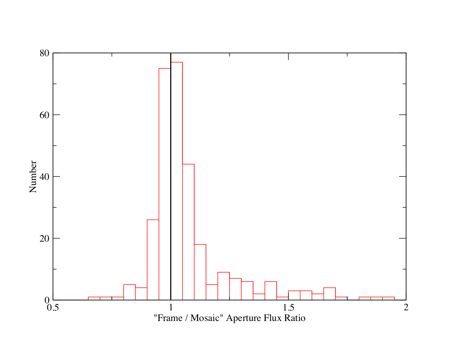
Figure 4a - Distribution of aperture flux differences: frame - mosaic (summed MJy/sr). Click to enlarge.
Figure 4b - Distribution of aperture flux ratios: frame/mosaic. Click to enlarge.
5. Impact of Masked (Missing) Pixels
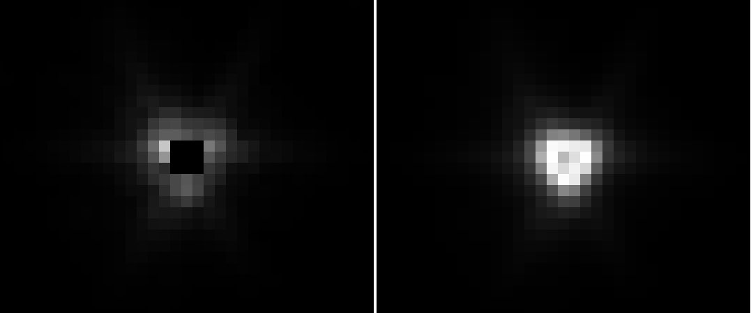
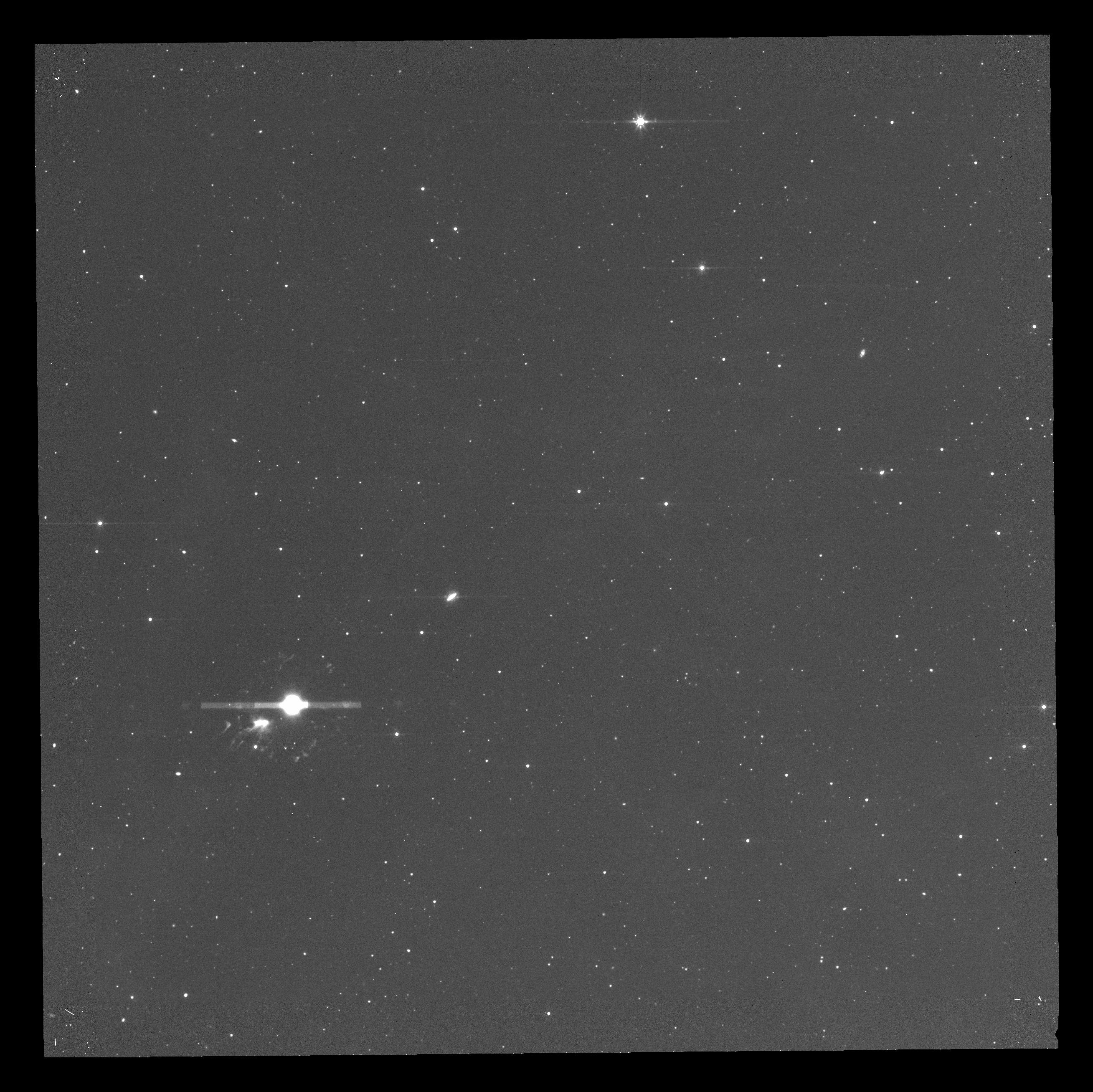
Figure 13 - Images of a bright star with a saturated core.
This star is located at top right in the IRAC band-1
mosaics of section IV.3.1.
Image on the left is from the
MOPEX mosaic
where the central
core pixels are NaN'd (entirely missing). Image on the
right is from the
AWAIC mosaic
where a significant fraction of flux in the core is recovered.
Click on image to enlarge.
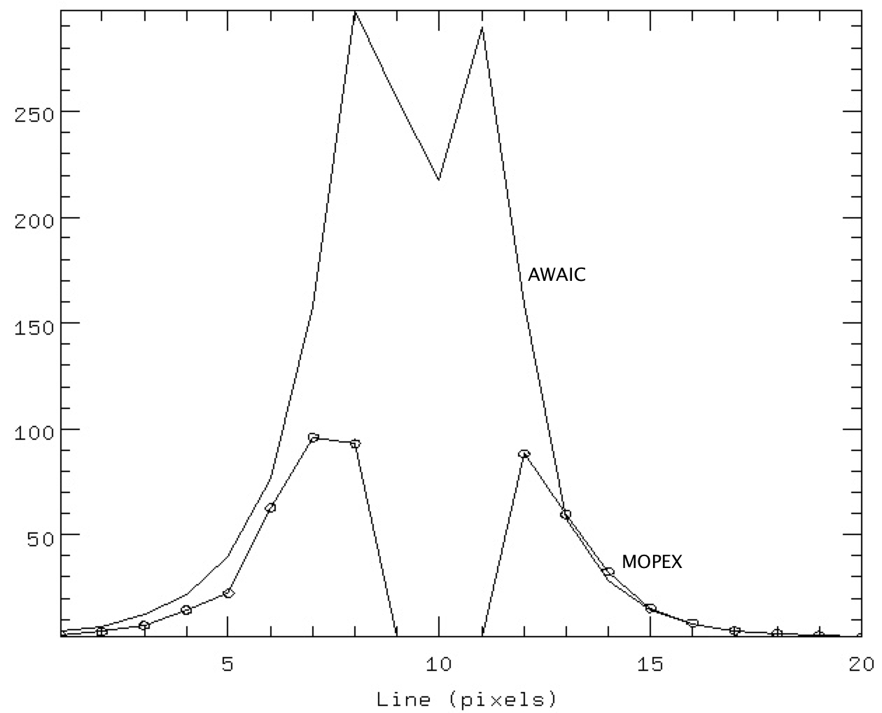
Figure 14 - pixel-row profile cuts centered at the
bright star cores shown in Fig. 13. The
MOPEX profile has "missing flux" at the core while the
AWAIC case recovers at least 70%.
Click on image to enlarge.
6. Examples of Resolution Enhancement
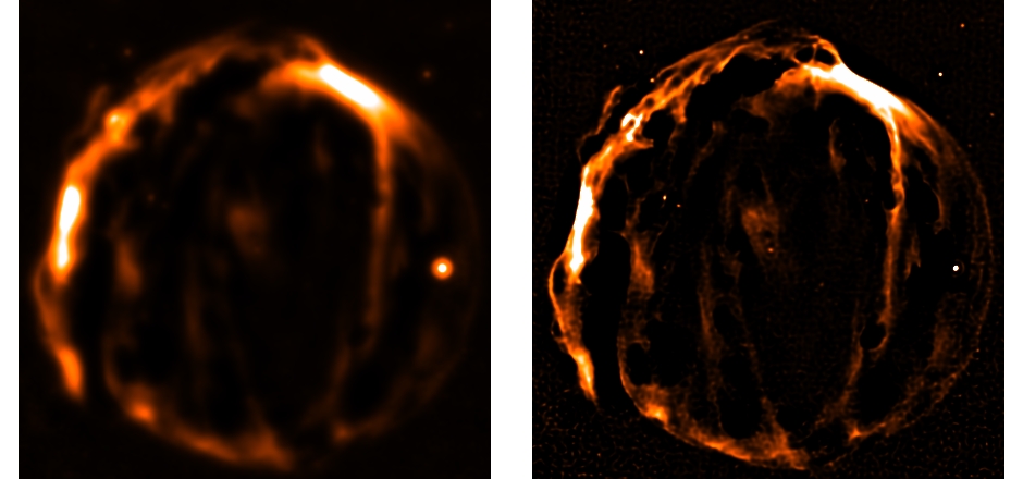
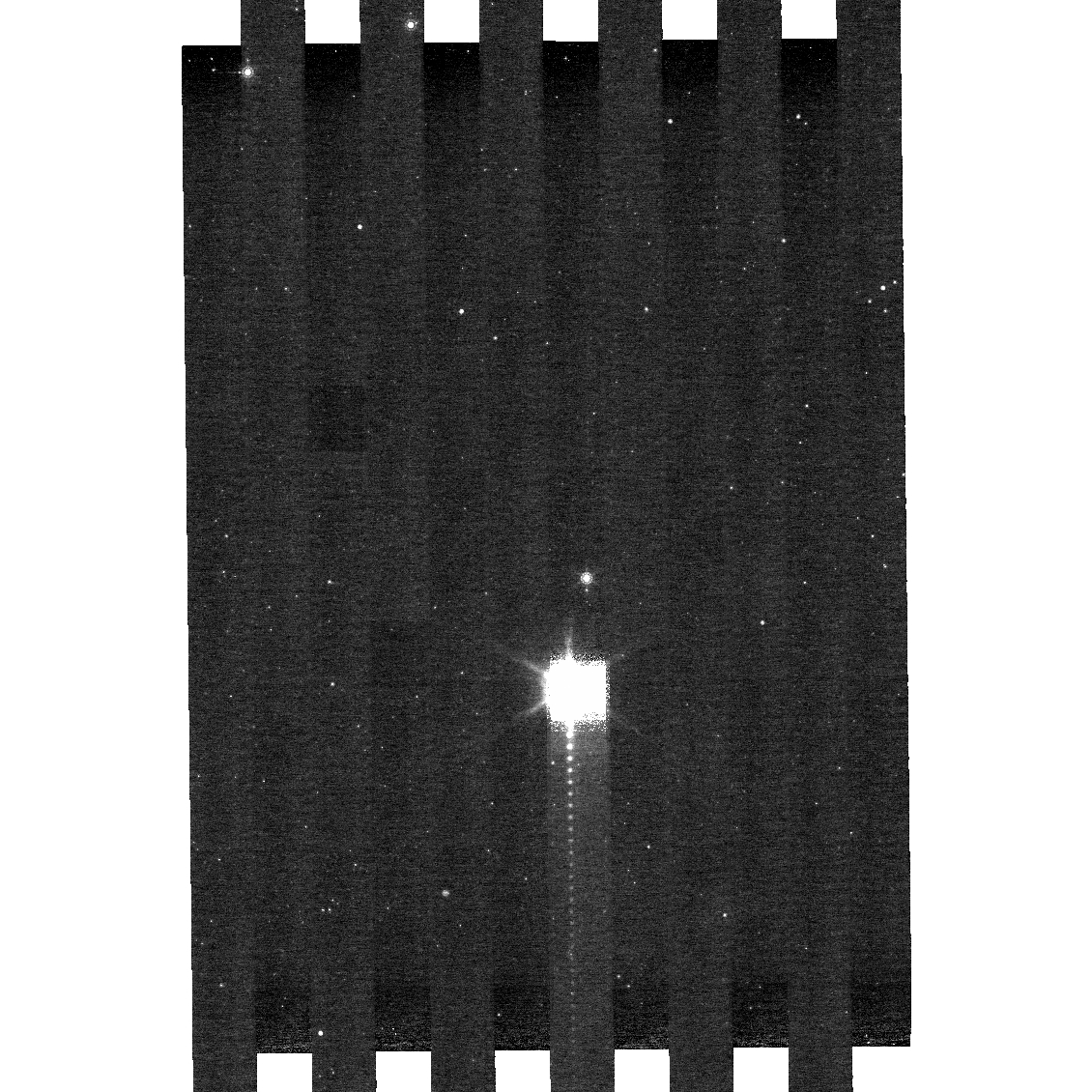
Figure 15 - Tycho's Supernova Remnant. Left:
simple co-add from AWAIC (after 1 iteration).
Right: HiRes'd version from AWAIC after 40 iterations.
Click on panel to enlarge.
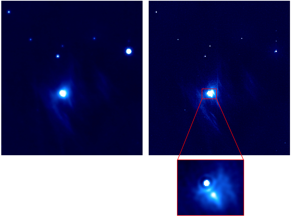
Figure 16 - A 13.6′ x 15′ star forming
region in Taurus from the
Taurus-2 Spitzer Legacy Program. Left:
simple co-add from AWAIC (after 1 iteration).
Right: HiRes'd version from AWAIC after 20 iterations.
See Figure 17 for depth-of-coverage and outlier maps.
Click on panel to enlarge.
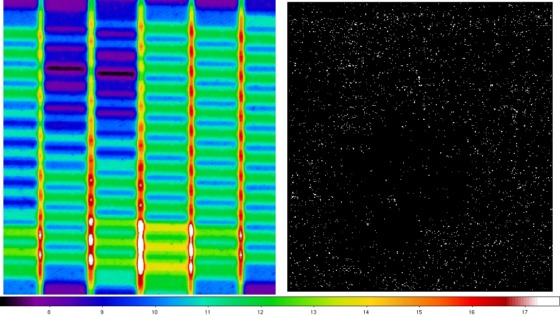
Figure 17 - Ancillary products corresponding to Figure 16.
Left: depth-of-coverage map with approximate
depths shown by color bar. Right: outlier map from
AWOD
where a white dot
indicates at least one pixel in the stack was contaminated
by an outlier. Click on panel to enlarge.
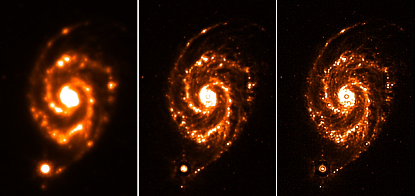
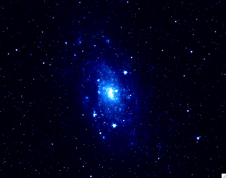
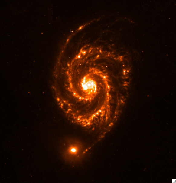
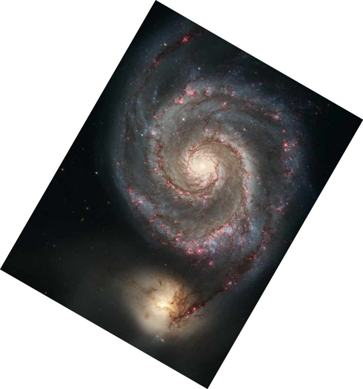
Figure 18 - NGC 5194/5195 or M51a/b.
Left: simple co-add from AWAIC (after 1 iteration).
Middle: HiRes'd version after 10 iterations.
Right: HiRes'd version after 40 iterations.
The ringing artifacts around the satellite dwarf galaxy
at the bottom
in the HiRes images arise because the core is saturated in the
data and the PRF is not a good match.
Other point-source ringing artifacts are due to
sources superimposed on the extended structure of the galaxy
and the inability to reconstruct their signal at high spatial
frequencies due to the band-limited nature of the measurements.
For comparison, an unHiRes'd co-add at 5.8μm (from IRAC)
is shown here, and
an optical image from HST is
here.
The FWHM of the effective PRF went from ~6 arcsec to ~2 arcsec
in the HiRes image, i.e., similar to that of the
IRAC 5.8μm detector. Click on panel to enlarge.
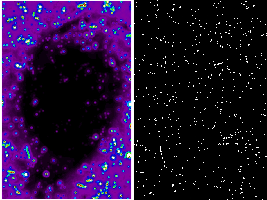
Figure 19 - Ancillary products corresponding to Figure 18.
Left: the MCM Correction Factor Variance (CFV)
after 40 iterations from AWAIC with no prior outlier masking.
This is the variance
corresponding to the PRF-weighted average correction factor in
Eq. 4. High values of the CFV imply an inconsistency
of the input measurements, e.g., outliers
(which were not masked here for the purpose of this
illustration). The CFV reacts to the fraction
of "outlier flux" relative to the expected signal, and that
fraction is usually less where the signal is
strong (e.g., on the galaxy itself).
Right: outlier map from AWOD.
As expected, there good
correlation with the CFV image.
Click on panel to enlarge.
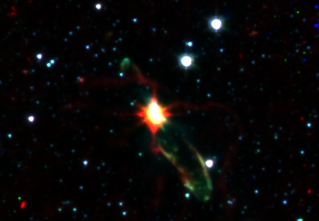
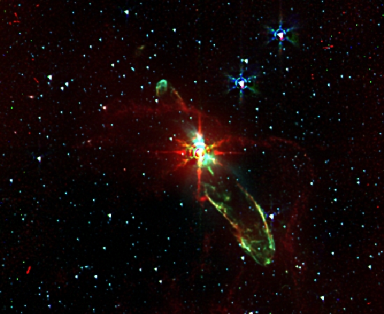
Figure 20 - Spitzer-IRAC false color composites of
Herbig-Haro 46/47:
3.6μm,
4.5μm,
8.0μm.
Left: combines co-adds from AWAIC (after 1 iteration).
Right: HiRes'd version from AWAIC after 20 iterations.
The ringing artifacts around the bright stars are due to
their profiles being slightly broader (e.g., "flattened
cores" due to saturation) than the input PRFs used for the
HiRes'ing. Click on a panel to enlarge.
V. Quantitative Analysis
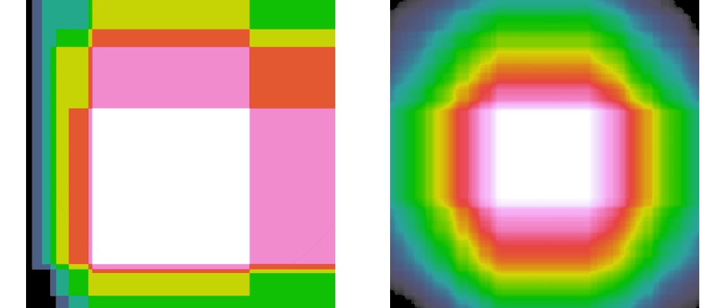
Figure 21 - depth-of-coverage maps for two sets
of simulated co-adds. Left: 16-frames;
Right: 256 frames. The central
(white) portions contain the maximum depths.
Click on image to enlarge.
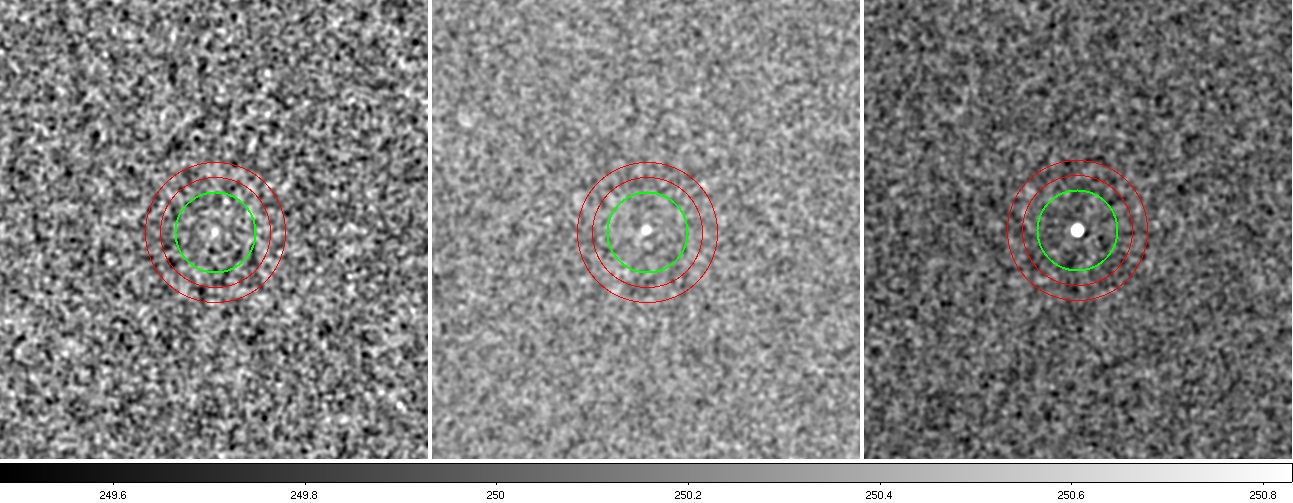
Figure 22 - simulated co-adds from AWAIC corresponding
to maximum central coverage depths
of 1 (left, i.e., a single interpolated frame),
8 (middle), and 256 (right).
The green circle is a test aperture
for our aperture photometry and the red
annulus is for the background estimation.
These are centered on our "known" simulated point source
which is barely visible on the "1-frame co-add".
Click on image to enlarge.
1. Co-add Pixel Uncertainties
(Eq. 8)
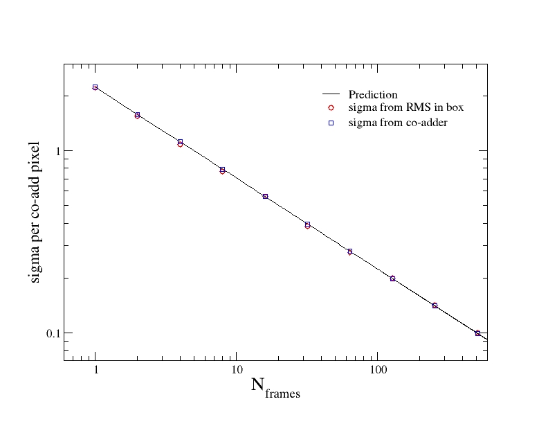
Figure 23 - Co-add pixel 1-sigma uncertainty as a function
of the number of frame-overlaps (1 to 512 frames).
The solid line is that
predicted by our simulation setup (Eq. 8).
The squares are the pixel uncertainties computed
by AWAIC (Eq. 7) and are constant
over space since we assumed a uniform background.
The circles correspond to the RMS
of pixel fluctuations in a box placed
on the background of each co-add.
The noise per co-add pixel scales as expected:
~1/√Nf (Eq. 8).
Since this is a log-log plot, the slope
of the solid line is -0.5.
2. Aperture Photometry and Correlated Noise
(Eq. 9)
(Eq. 10)
(Eq. 11)
(Eq. 12)

(Eq. 13)
 |
(Eq. 14) |
Figure 24 shows the result of our aperture photometry as a function of the number of frame-overlaps in a co-add. Eqns 11 - 13 were used to estimate fluxes and uncertainties. The 1-sigma error bars account for correlated noise in the source aperture as well as the background annulus. The correlation correction factors, Fcorr(NA) and Fcorr(NB), were first computed numerically from the PRF. With NA ~ NB, we found values of ~6 for both factors. These were then verified by placing 500 apertures at random within co-add regions with uniform coverage and computing the RMS of their total fluxes. This effectively gave the total uncertainty sought for, but, when divided by the uncorrelated RSS'd pixel sigmas (e.g., sum term in Eq. 11), factors of 6±0.3 were found, in agreement with our numerical estimate.
In the end, ignoring correlated noise
would have lead us to underestimate source-flux errors and
hence overestimate signal-to-noise ratios
by a factor of ~6. This example shows the danger of
ignoring correlated errors when determining photometric accuracy
off a co-add made using an interpolation kernel spanning
many pixels. This holds for both aperture and profile
fitting methods when applied directly on a co-add.
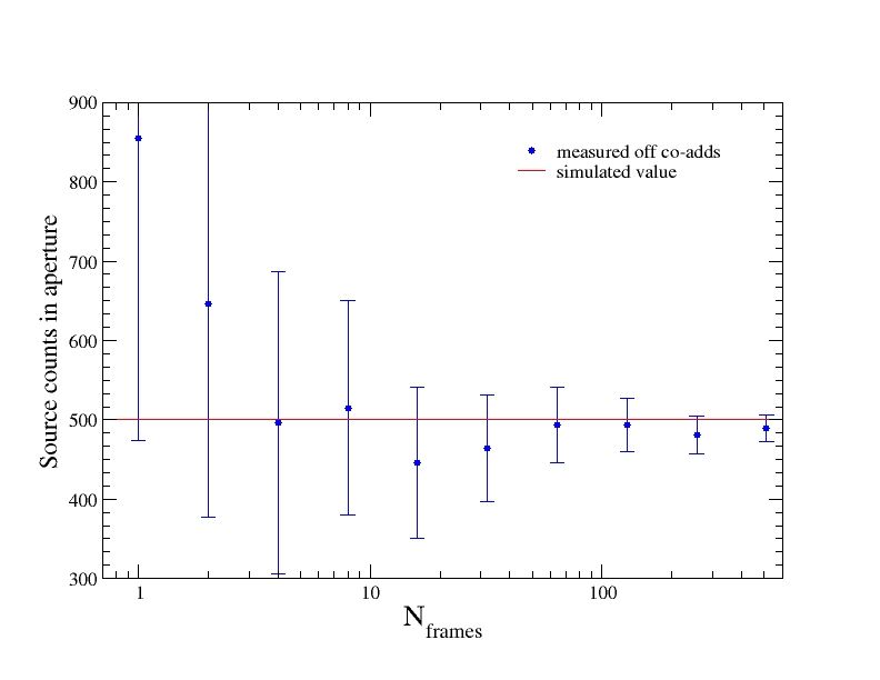 |
| Figure 24 - Total background-subtracted counts ("flux") in an aperture centered on our point source versus number of frame-overlaps in co-add. The solid horizontal line is the "truth". Overall, the measured counts are repeatable to within measurement error across all co-add depths. The error bars are all 1-sigma and account for spatial correlations between pixels (see section V.2). |
The author is indebted to Gene Kopan, John Fowler and Ken Marsh
for illuminating and philosophical discussions.