
| AWOD: A WISE Outlier Detector | |
We present some preliminary results from the WISE (temporal) outlier detector - AWOD. The plan is to execute this module prior to frame co-addition with AWAIC. Its primary goal is to detect "out-of-bed" frame pixels (with significantly inconsistent measurements) at the same location on the sky and record them in pixel masks for use downstream (e.g., source photometry). Potential outliers include cosmic rays, latents, other optical/instrumental artifacts, supernovae!, asteroids, and basically anything that has moved or varied appreciably with respect to the inertial sky (e.g., the CMB) over the observation span of all overlapping frames. This also includes inconsistencies due to poor frame registration, e.g., pointing errors greater than the typical size of a native pixel.
In a nutshell, AWOD performs its task by first reprojecting and interpolating each frame onto a common upsampled grid, then it uses robust statistics on each pixel in the grid-stack to detect outliers. The robust metrics used are the median and the Median Absolute Deviation (MAD) from the median as a proxy for sigma. An adaptive thresholding technique is used where thresholds are inflated at the location of "real" sources (by a predetermined amount) to avoid flagging pixels therein. The interpolation is performed using a top-hat PRF kernel. This accentuates and localizes the outliers for optimal detection (for instance, cosmic rays). Algorithmic details are decribed in the Software Design Specification document.
We tested AWOD on a set of 70 band-1 simulated frames provided by Ned Wright. Details of this simulation can be found here. Figure 1 shows an outlier map (left) from AWOD, and the corresponding mosaic from AWAIC (right) with the proposed dimensions of a WISE Atlas Image. The region represented here is a cut-out centered on the overall simulation.
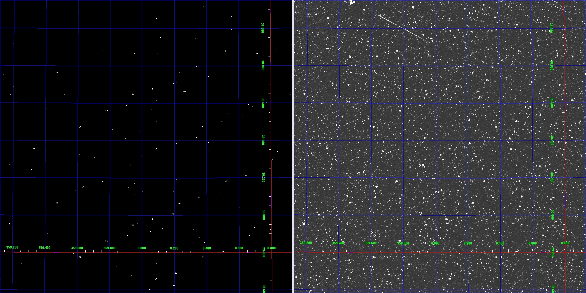 |
| Figure 1 - Left: Outlier map (8-bit mosaic) from AWOD with white indicating that an outlier was detected in at least one of the frames in the stack at that location. Right: Atlas Image mosaic of the same region spanning ~1.56° x 1.56°. The coordinate grid overlays are in the ecliptic system. The streak at the top is a diffraction spike artifact from the 2MASS catalog. The offending star is Beta Pegasi. Click on panel to enlarge. |
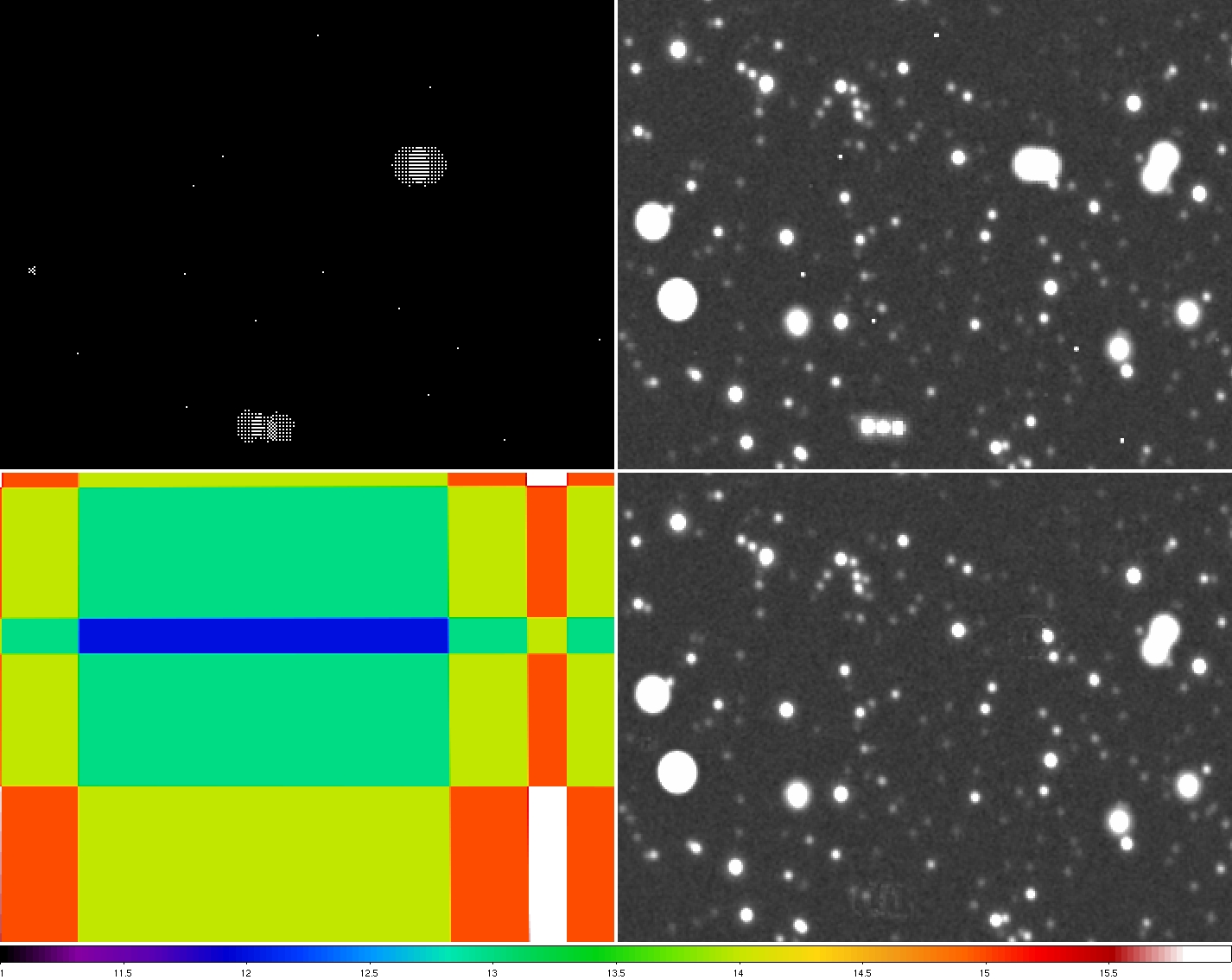 |
| Figure 2 - Top left: Outlier map of a zoomed-in region known to contain simulated latents and cosmic-rays. Top right: co-add of same region with no outlier rejection. Bottom left: corresponding depth-of-coverage map. Bottom right: co-add with the prior-masked outliers rejected. Both the outlier corrected and uncorrected co-adds were created using overlap-area weighting (top-hat PRF interpolation). Click on panel to enlarge. |
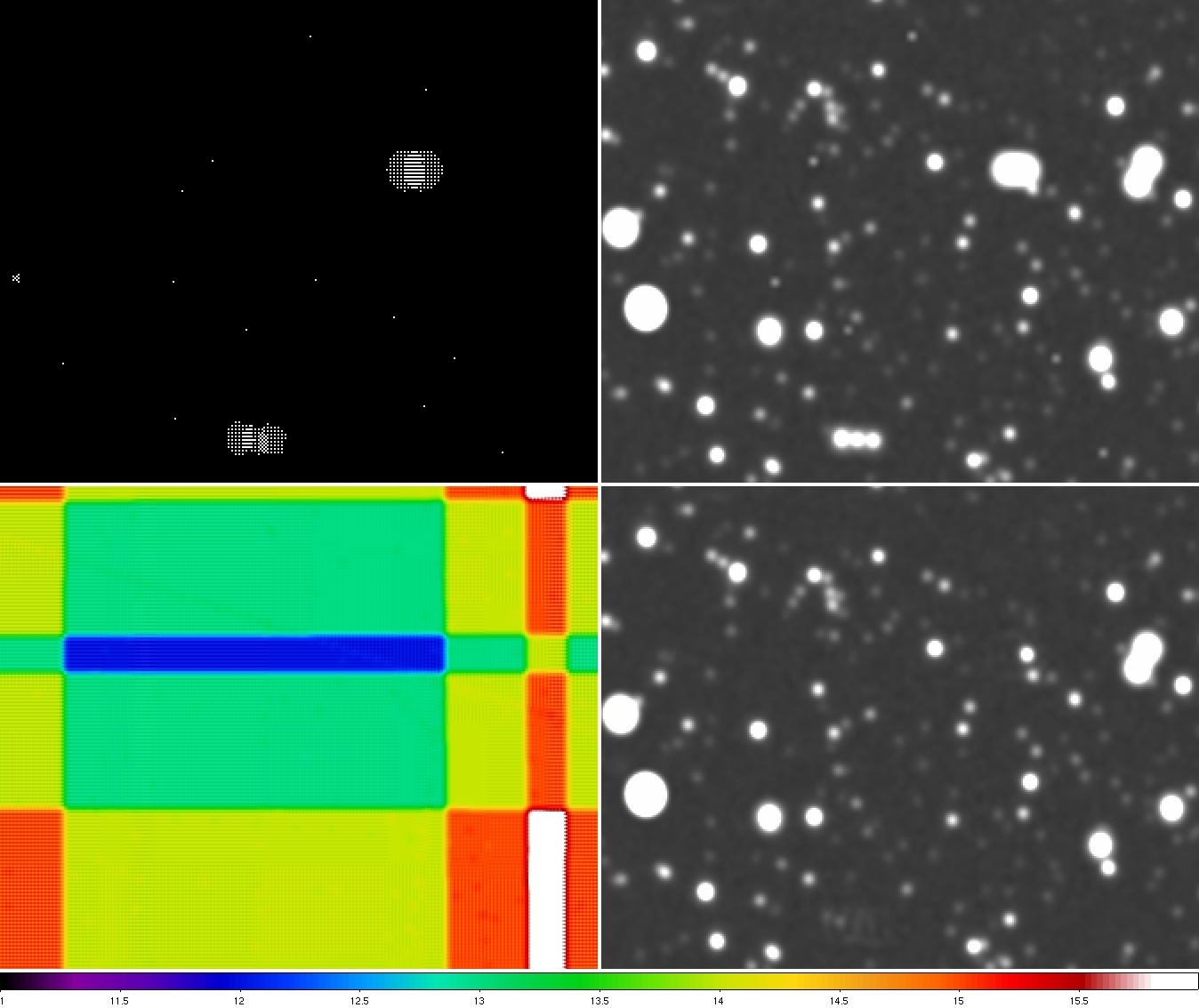 |
| Figure 3 - Top left: Outlier map of a zoomed-in region known to contain simulated latents and cosmic-rays. Top right: co-add of same region with no outlier rejection. Bottom left: corresponding depth-of-coverage map. Bottom right: co-add with the prior-masked outliers rejected. Both the outlier corrected and uncorrected co-adds were created using a broad PRF as the interpolation kernel. Click on panel to enlarge. |
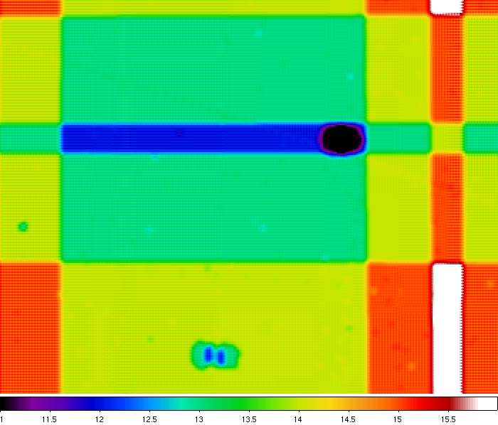 |
| Figure 4 - Depth-of-coverage map corresponding to the outlier-rejected PRF-interpolated co-add in Figure 3. Note the reduced depths at the flagged outlier locations. Click on panel to enlarge. |
We simulated 100 randomly dithered, overlapping frames containing a constant background of 1000 counts per pixel. Poisson noise was added to each frame pixel by sampling from a normal distribution with variance equal to the mean background. 500 single pixel cosmic ray hits were then randomly added to each frame. Their strengths were sampled from a uniform distribution spanning ~5 to 30σ from the mean background (where σ = √1000 ~ 31.6). To examine the dependence of outlier detection statistics on the depth-of-coverage, sets of 8, 16, 32 and 64 frames were fed into AWOD. The upper-tail flagging threshold was also varied. The detected outliers were then enumerated and compared against the truth list to compute the completeness and reliability.
Results are summarized in Figure 5. As expected, the reliability increases (and completeness decreases) as the threshold increases at a fixed depth-of-coverage. At a fixed nominal threshold, both reliability and completeness decrease with decreasing depth-of-coverage. This is due to the sigma estimates becoming more unreliable (noisier themselves) as the frame stack-size decreases.
It's important to note that this simulation is far from reality. The inclusion of sources will certainly impact the outlier statistics. The only source of "unreliability" in our simulation are noise spikes. This exercise merely served to check that the module performs as expected for different assumed thresholds and coverage depths.
A similar analysis using the 70-frame mid-latitude simulation from
above is pending. Cosmic ray truth lists, and a scheme to
distinguish between these and latent-source outliers (and possibly
moving objects too) are first needed.
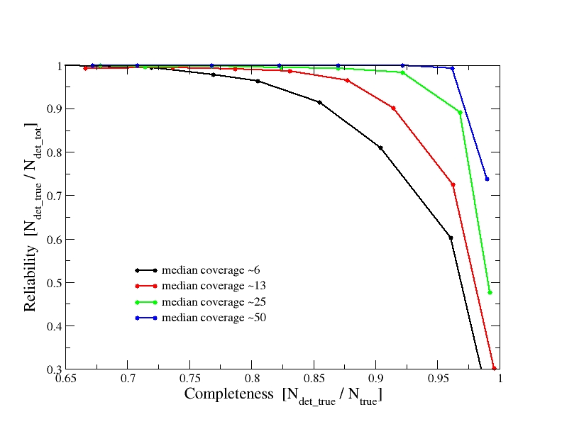 |
| Figure 5 - Reliability versus Completeness for the "superficial" simulation described in section 3. Results are shown for four median coverage depths. The dots on each curve going from right to left correspond to detection thresholds of 3, 4, 5, 6, 7, 8, 9 and 10σ. |