


i. Overview
1. Sky Tiling and Footprint Definition
ii. Throughput (Gain) Matching
iii. Frame Overlap/Background-level Matching
iv. Flagging Moon-affected Frames Using Prior Mask
1. Prior Moon-masks
2. Moon-contamination Processing
v. Pixel Outlier Detection and Masking
1. First-Pass Computations
2. Second-Pass Computations
3. Outlier Expansion
vi. Frame-Based Rejection
vii. Frame Co-addition using PRF Interpolation
The Atlas Images were generated using AWAIC: A WISE Astronomical Image Co-adder. This is a software tool custom built for WISE. It performs the following primary functions when combining the multiple frame exposures that overlap a specific sky footprint:
The goal of image co-addition in AWAIC is to optimally combine a set of (usually dithered) exposures to create an accurate representation of the sky, given that all instrumental signatures, glitches, and cosmic-rays have been properly removed. By "optimally", we mean a method which maximizes the signal-to-noise ratio (SNR) given prior knowledge of the statistical distribution of the input measurements. Figure 1 gives an overview of the main steps in AWAIC. The co-addition step is shown in the red box. We expand on the main steps below.
It is assumed the input science frames were preprocessed to remove instrumental signatures and their pointing reconstructed in some World Coordinate System (WCS) using an astrometric catalog. Accompanying bad-pixel masks and prior-uncertainty frames are also used. A bit-string is also specified on input to select which bad-pixel conditions to mask and omit from co-addition. Prior to co-addition, frames are filtered according to whether any were too close to an anneal (nominally 2000 sec; see V.2.c), had a bad quality score (from frame-level QA), or were part of dedicated experiments throughout the mission. Section V.2.c summarizes the frame selection criteria.
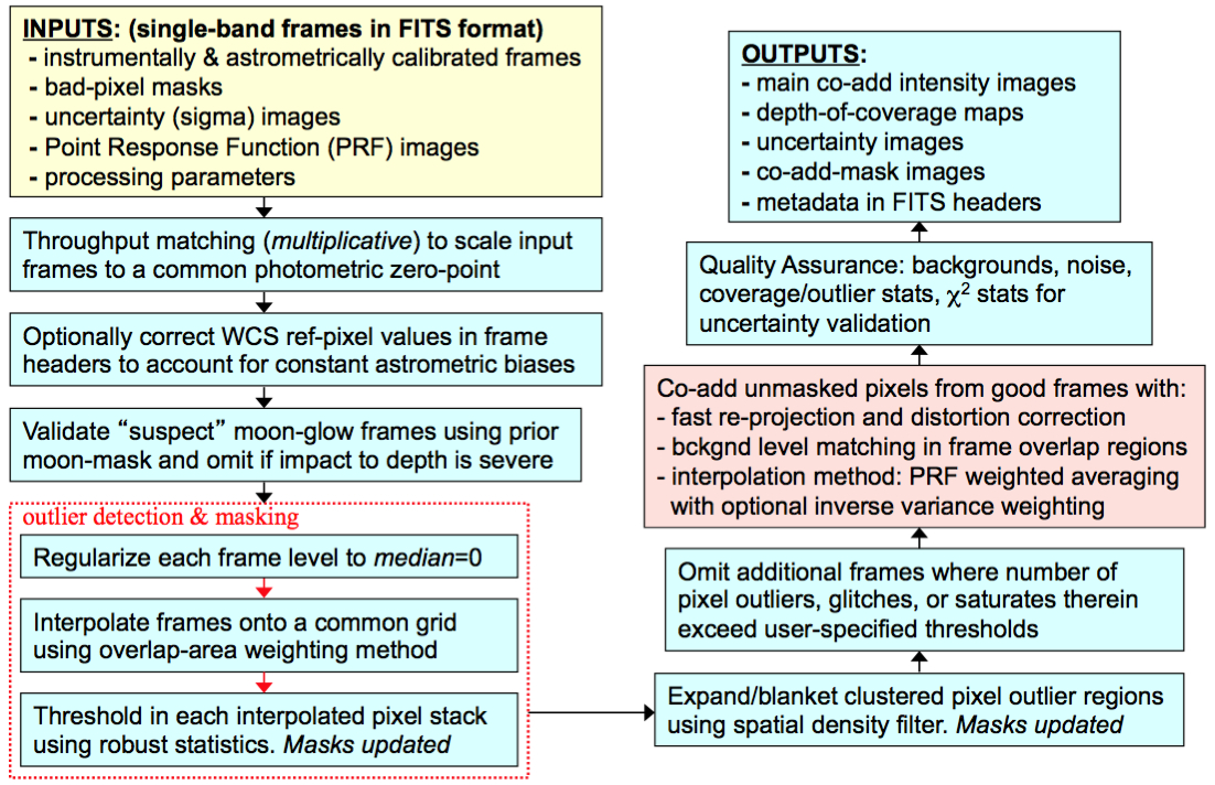 |
| Figure 1 - Processing flow in the WISE co-adder: AWAIC. |
The input frames are assumed to overlap with some predefined footprint on the sky. This footprint also defines the dimensions of the Atlas Image products: ≈ 1.56444o x 1.56444o or 4095 x 4095 pixels with a linear plate scale of 1.375″/pixel at the center. 1.56444o is the approximate projected linear scale after orthographically ("SIN") projecting the sky onto an Atlas Image plane.
The Atlas Image footprints were defined using a simple tiling geometry whereby the tiles were optimally arranged in separate iso-declination bands assuming a minimum linear overlap of 3 arcmin at the celestial equator. This overlap increased towards an equatorial pole (e.g., see Figure 2) and was tweaked within each declination band to obtain a uniform distribution of tile spacings. All tiles were assigned a position angle relative to equatorial north of zero. The WCS of all WISE Atlas Image footprints, i.e., their center RA, Dec and corner coordinates can be found in Table 1:
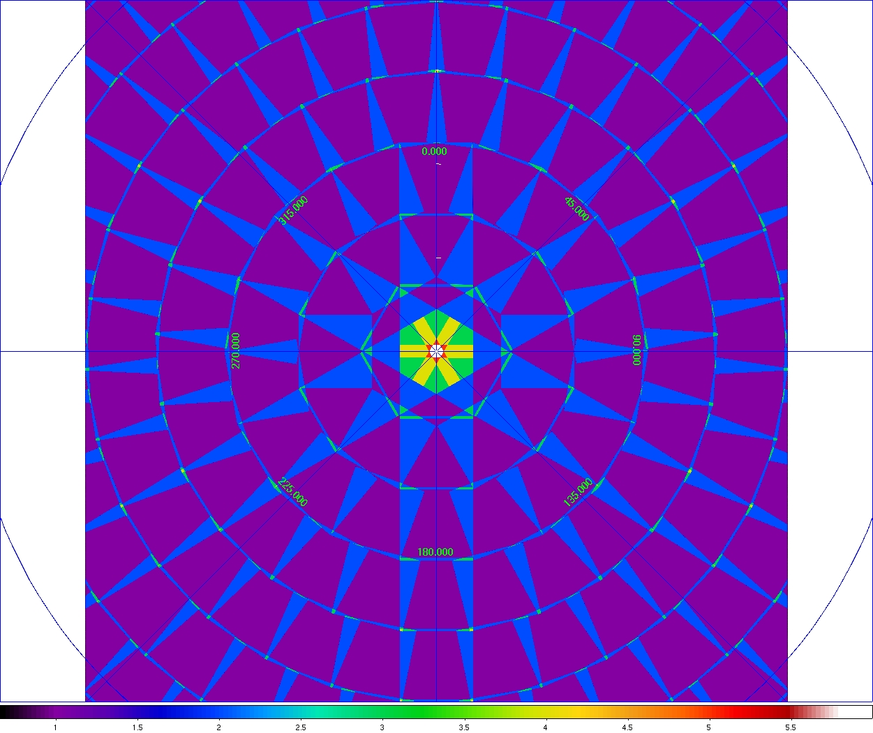 |
| Figure 2 - Layout of Atlas Image footprints at an equatorial pole. Color-bar shows the number of overlaps at any point. |
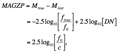
The first step was to scale the frame pixel values to a common photometric zero-point using calibration zero-point information stored in the MAGZP keyword of each input frame FITS header. MAGZP is defined as:
 |
(Eq. 1) |
where Mtrue and Minst are the true and instrumental magnitudes of a calibrator source respectively; DN (Data Number) are the raw image pixel counts of the calibrator source from photometry (with background subtraction); ftrue is its true flux density (e.g., Jy); f0 is the flux corresponding to magnitude zero (see also Table 1 in II.3.f), and c = ftrue/DN = the DN-to-[Jy] conversion factor (or whatever absolute units are desired).
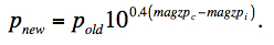
We shall label the MAGZP in an input frame FITS header as magzpi. Given a common (or target co-add) zero-point magzpc, the pixels (pold) in frame i are rescaled according to:
 |
(Eq. 2) |
The same operation is performed on the input uncertainty frames. The target zero point (magzpc) is then written to the Atlas Image FITS header as MAGZP. This enables the calibration of photometric measurements off a co-add (see II.3.f). An accompanying uncertainty "MAGZPUNC" is also written to the Atlas Image FITS header, initially derived from photometric calibration. The MAGZP and MAGZPUNC values are the same for all Atlas Images of a given band and are summarized here.
Frame exposures taken at different times usually show variations in background levels due to, for example, instrumental transients, changing environment, changing zodiacal emission with orbital position, scattered and stray light. The goal in background-level matching was to obtain seamless (or smooth) transitions between frames near their overlap regions prior to co-addition, but at the same time preserving natural background variations and structures on local scales as much as possible. Given the WISE mission had no requirements on the background, we adopted a simple locally self-consistent method. Only the single exposure frames touching an individual Atlas Image tile (independent of all those touching neighboring tiles) were matched with respect to each other. Caveats of the method are discussed further below.
The frame-overlap level matching is performed in-situ as each frame
is dynamically reprojected and interpolated onto the output
co-add footprint in AWAIC. It entails first computing the difference
in the median values of pixels in the (common) overlap region
between an incoming frame and those already in the co-add footprint
(if any exist from previously reprojected frames). Let's label this
constant overlap difference as
Δinput ∩ coadd. Before the input
frame pixels are interpolated and added onto the output co-add grid,
this difference is subtracted from all of its pixels
pij(old frm):
 |
(Eq. 3) |
for overlapping pixels on the sky with common coordinates α, δ. This process is applied to all the input frames and ensures continuity in background levels across their overlap regions. As a detail, if there are no or too few pixels in the overlap region between an incoming frame and those already in the co-add (according to some threshold), the median of all coadd pixels containing a real flux from previous frame reprojections is subtracted from the full-image median of the incoming frame.
According to the above process, the final background level in a co-add is dictated by the first frame that was reprojected since all subsequent frames will be level-matched in succession with respect to what is already in the co-add footprint. The first frame therefore sets the course for all other frames and could itself have a background that is anomalous or not globally representative of all the input frames. We therefore regularize the final coadd background level by first subtracting the mode of all its pixels, then adding the global median of all the original input frame pixels.
One can envisage extending the above formalism and fitting a tilted 2D plane (or even a surface) to pixel differences in the frame-to-coadd overlap region. Besides substantial increases in processing time, we found this to be unnecessary in general for WISE. We have assumed the difference in levels in the overlap region between any pair of frames is spatially constant.
Two caveats of the above method (also outlined in cautionary note I.4.c.v) are:
A flowchart for eliminating frames (severely) contaminated by scattered moon-light is shown in Figure 5. Here we expand on some of the details. The method uses an input moon-frame metadata table that stores information on which input frames contain suspect moon-glow according to a moon-centric all-sky mask made from offline analysis. This is described in section iv.1. The moon flagging process in described in section iv.2 below.
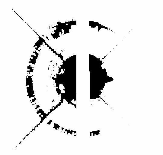
The moon-centric masks were made by thresholding on a robust pixel-variance metric for all frames acquired during the first five months of the mission. Frames within the galactic plane were excluded. Given W3 and W4 were the most heavily affected by moon glow, only masks for these bands were made. In the end, we adopted the same mask for W3 and W4. The raw mask for W3 (~similar to W4) is shown in Figure 3. We assumed simple symmetric masks for W1 and W2 based on an exclusion radius. This radius was empirically tuned to avoid the worst moon artifacts. For completeness, the W3 and W4 masks were then smoothed to fill in the fuzzy diffraction pattern-like regions. The smoothed moon masks used in processing are shown in Figure 4.
 |
 |
| Figure 3 - Raw (unsmoothed) mask in the moon-centered reference frame derived from W3 data (the W4 mask is similar). Black denotes regions where frames are suspected to be badly contaminated by moonlight. | Figure 4 - Smoothed moon-masks for each band used in multiframe processing. |
The prior moon masks determine whether a frame contains suspect moon glow. This is considered "suspect" because many of the frames could still proceed downstream to the outlier detection step for further dissemination and filtering (see below). Furthermore, the input moon-masks could be aggressive and the existence of slight moon glow could not be detrimental when combined with other good frames. This ensures that the S/N is optimized in the final coadd. A blind rejection of all suspect moon-glow frames will leave large holes in the survey. The suspect moon frames tagged in the input moon-metadata table are therefore further filtered using robust spatial metrics as follows.
We compute robust measures of the spatial pixel RMS for both the suspect moon-masked frames and non-masked frames. The former is expected to be larger than the latter due to the presence of (usually non-uniform) moon glow. Note that elevations in background levels due to sptially uniform moon-glow are not detrimental to co-addition. This is another reason for post-filtering the suspect moon-glow frames. Simple elevations in background may have been removed by the background-matching step anyway. It's the fast-changing high spatial frequency variations that could cause problems. The distribution of RMSs for the non-masked frames is assumed to be representative of the normal "good" frames touching the coadd footprint, and serves as a benchmark against which the moon-masked frames can be validated for genuine moon-glow (see below). The robust RMS is computed using the median - 16th percentile of the pixel distribution in each frame.
As indicated in the third box down in Figure 5, we declare a suspect moon-glow frame as containing significant and detrimental moon-glow if its RMS is greater than some threshold of the RMS distribution of normal good frames. If no normal (unmasked) frames were present in the moon-metadata table, then both their median and spread in RMS are set to zero so that all suspect moon-frames are declared as "bad". This is a conservative approach although it rarely happens since the moon-toggling maneuver in the WISE survey causes a pile-up of frames (with factors of ~2 - 3 increase in depth-of-coverage) whenever the moon is near, and unmasked frames almost always trickle through. There are handful of cases however where all of the input frames touching a footprint fall very close to the moon warranting all of them being thrown out from further processing. Holes in the survey due to severe moon-glow are therefore inevitable (see cautionary notes in section I.4.c).
Once the genuine (or worst) moon-glow frames are identified, we build a coarsely sampled depth-of-coverage map using only these frames (e.g., 100 x 100 bins). We also build a depth-of-coverage map including all frames (masked + unmasked + not rejected for other reasons upstream). We then take the ratio of the moon-only depth map to the total depth map to make a moon depth-fraction (or mdf) map. This is used in the next step to decide if the moon-depth is overall too high for the pixel-outlier rejection step downstream to operate reliably.
If the mdf is too high, all the moon-glow frames (the post-filtered "genuine" set) are rejected from downstream processing. If not, they proceed to the outlier rejection step for further dissemination at the pixel level. This process ensures that the coadd S/N is maximized. In general, the pixel-outlier algorithm requires that no more than ~50% of a pixel stack (after interpolation) be comprised of outliers for them to be reliably detected and rejected (for details see section v.). If greater than ~50%, these "outliers" become the norm for the coadd signal and no outliers will be detected based on the use of median statistics. Biases will then result in the final coadd. Therefore, 50% is the breakdown point before we can be confident that outlier rejection can deal with any remaining moon-contaminated pixels. Formally, all moon-glow frames are rejected if the mdf exceeds some threshold mfrac (default = 0.5) over a region greater than some fraction of the footprint area (default fraction = 0.001 or 10 mdf pixels for a 100 x 100 sampled grid).
As a detail, if these thresholds are not satisfied and moon-contaminated frames do proceed to the pixel-outlier detection step, the depth in any interpolated pixel stack needs to exceed a minimum of 4 to have a fighting chance at being reliably detected and rejected. Note that "reliably detected" is a fuzzy term since in general, outlier detection is a noisy process when the depth-of-coverage is low to moderately low, e.g., < ~ 6. To avoid throwing away many good pixels, no outlier detection whatsoever is performed if the depth is ≤ 4. Therefore, if any moon-contaminated frames are passed onto the outlier detection step (after all the above post-filtering) and the total depth is relatively low (e.g., < ~ 6), it's possible to end up with moon-contamination in a co-add. This will always be true if the depth is ≤ 4 since no outlier detection is performed as described.
The number of frames suspected to contain moon-glow (as determined from the prior moon-mask alone) is stored as the "MOONINP" keyword in Atlas Image FITS headers. Furthermore, the actual number of frames rejected (after the filtering described above) is stored as the "MOONREJ" keyword.
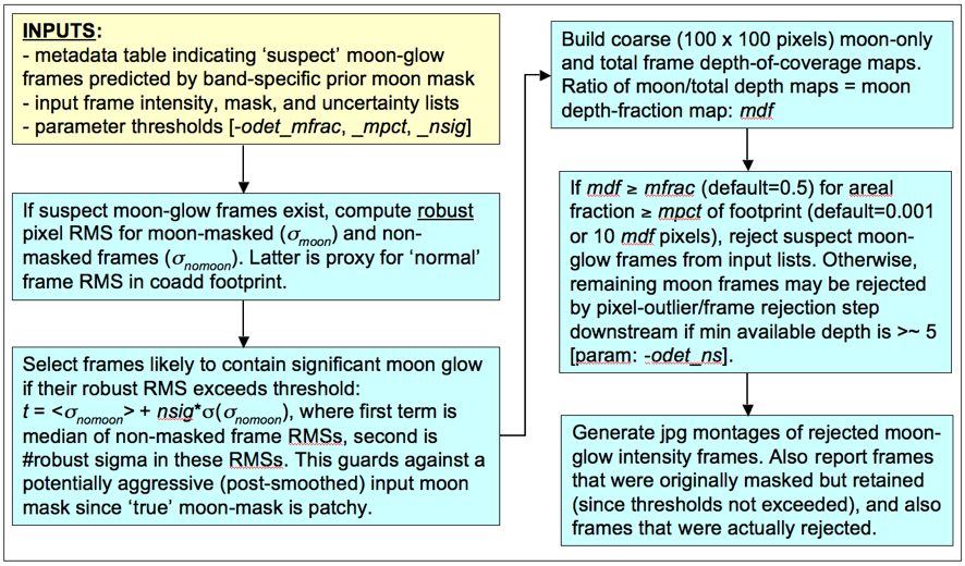 |
| Figure 5 - Processing flow for rejecting moon-contaminated frames. |
The goal of outlier detection is to identify frame pixel measurements of the same location on the sky which appear inconsistent with the (bulk) remainder of the sample at that location. This assumes multiple frame exposures of the same region of sky are available. Potential outliers include cosmic rays, latents (image persistence), instrumental artifacts (including bad pixels), poorly registered frames from gross pointing errors, supernovae, asteroids, and basically anything that has moved or varied appreciably with respect to the inertial sky over the timespan of the input frames. Outlier detection and flagging is executed by the AWOD module (A WISE Outlier Detector) - called from the same script as AWAIC.
In summary, the method first involves projecting and interpolating each input frame onto a common grid with user-specified pixel scale optimized for the detector's Point Spread Function (PSF) size. The interpolation is performed using the overlap-area weighting method (analogous to using a top hat kernel). This accentuates and localizes the outliers for optimal detection (e.g., cosmic ray spikes). When all frames have been interpolated, robust estimates of the first and second moments are computed for each interpolated pixel stack j. We adopt the sample median (med), and the Median Absolute Deviation (MAD) as a proxy for the dispersion:
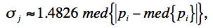 |
(Eq. 4) |
where pi is the value of the ith interpolated pixel within stack j. The factor of 1.4826 is the correction necessary for consistency with the standard deviation of a Normal distribution in the large sample limit. The MAD estimator is relatively immune to the presence of outliers where it exhibits a breakdown point of 50%, i.e., more than half the measurements in a sample will need to be declared outliers before the MAD gives an arbitrarily large error. The second step involves re-projecting and re-interpolating each input pixel again, but now testing each for outlier status against other values in its stack using the pre-computed robust metrics and thresholds for its distance below or above the sample median. If an outlier is detected, a bit is set in the accompanying frame mask so the pixel can be omitted from co-addition downstream.
We require typically at least five samples (overlapping pixels) in a stack for the above method to be reliable. This is because the MAD measure for s, even though robust, can itself be noisy when the sample size is small. Simulations show that for the MAD to achieve the same accuracy as the most optimal estimator of s for a normal distribution (i.e., the sample standard deviation), the sample size needs be ≈2.74x larger. Another requirement to ensure good reliability is to have good sampling of the instrumental PSF, i.e., at the Nyquist rate or better. When well sampled, more detector pixels in a stack can be made to align within the span of the PSF, and any pixel variations due to PSF shape are minimized. On the other hand, a PSF which is grossly under sampled can artificially increase the scatter in a stack, with the consequence of erroneously flagging pixels containing true source signal. WISE is marginally sampled at the Nyquist rate in all bands, so this possibility is reduced but not eliminated. Figure 6 illustrates these concepts.
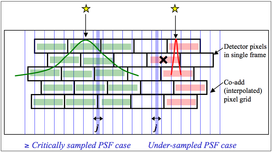 |
| Figure 6 - One-dimensional schematic of stacking method for detecting outliers for well sampled (left) and under-sampled (right) cases. The input pixel marked X contains signal from a source and is in danger of being flagged when outlier detection is performed at location j in the output grid. |
The outlier detection and rejection process is shown in Figure 7. Details of the two-pass process summarised above are expanded in sections v.1. and v.2.. Section v.3. outlines the outlier-expansion algorithm, designed for more complete masking of extended outliers with "fuzzy" edges, e.g., asteroids.
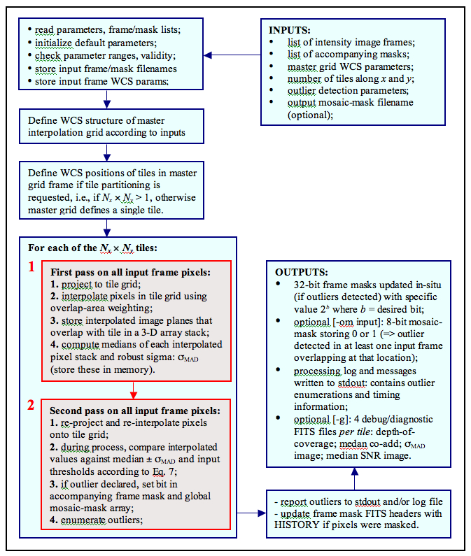 |
| Figure 7 - Processing flow in AWOD (A WISE Outlier Detector). Red boxes represent the main computational steps described in sections v.1 and v.2. |
The first pass projects frame pixels using a fast pixel-to-pixel WCS transformation onto the interpolation grid. This transformation also corrects for FOV distortion using the SIP FITS representation. The interpolation uses the overlap-area weighting method to compute the flux in the output grid pixels. In essence, this method involves projecting the four corners of an input pixel directly onto the output grid (with rotation included). Input/output pixel overlap areas are then computed using a textbook algorithm for the area of a polygon, and then used as weights when summing the contribution from the pixels of an input frame with signals Di. The signal in grid pixel j from frame k is given by:
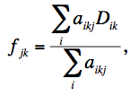 |
(Eq. 5) |
where aikj
is the overlap area between pixel i
from input frame k with output
grid pixel j (see schematic
in Figure 8).
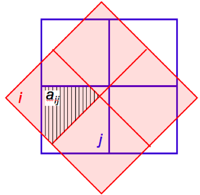 |
| Figure 8 - Schematic of overlap-area weighted interpolation used in Eq. 5. |
The projection and interpolation is only performed for frames that overlap with the footprint tile. This overlap pre-filtering is performed using a coarse method whereby an overlap is declared if the separation between the centers of a tile and input frame is less than the sum of the radii of circles that circumscribe the tile and frame. The interpolated planes for each overlapping frame are stored in a 3-D cube. Since the outlier detection and rejection process is memory intensive, the interpolated planes are stored as 16-bit integers using a scaled-logarithmic transformation of the input floating-point values. The robust stack estimators are computed using 16-bit arithmetic and transformed back to floating-point. The loss in precision is negligible.
The median is then computed for each interpolated pixel stack j by first sorting the pixel samples using the heapsort algorithm. The median is computed as the 50th percentile of the sorted stack, and we compute a robust measure of the dispersion that is an approximation to the actual σMAD defined by Eq. 4. This is a very good approximation and is designed for speed. It works directly off the sorted pixel stack stack[k] by selecting appropriate indices:
 |
(Eq. 6) |
where the factor 1.482.. is the correction to ensure Normality in the large sample limit and N is the stack depth. The array indices are rounded down to the nearest integer.
AWOD includes an adaptive thresholding method in that if it encounters a pixel that's likely to be associated with "real" signal (e.g., a source), then the upper and lower thresholds are automatically inflated by a specified amount to avoid (or reduce the incidence of) flagging such sources as outliers in the second pass (see below). To distinguish between what's real or not, we compute a median SNR image corresponding to the interpolated pixels j. This is computed using:
 |
(Eq. 7) |
The first term in the numerator of the SNR expression in Eq. 7 is the median signal for pixel stack j, and the second term is a global background measure. This background is computed as the median signal over all stack medians such that their depth-of-coverage Nj is equal to the median depth over the entire footprint. The denominator is an estimate of the spatial RMS fluctuation for pixel stacks at the median depth-of-coverage, relative to their median signal (the base RMS), and then appropriately rescaled to represent the pseudo-local RMS at any depth Nj (third line in Eq. 7). More precisely, the base RMS (last line in Eq. 7) is computed using the lower tail percentile values of the pixel distribution to avoid being biased by sources and other spatial outliers. The local SNR computed this way is an approximation and assumes the background does not vary wildly. The median SNR image is used for regularizing the σMADj image (see next paragraph) and is a proxy for real source pixel-signal to assist in the actual outlier flagging process (section v.2.).
We regularize (or homogenize) the σMADj values where they are too low relative to their overall neighboring values, or too high in regions below some minimum SNR (using the median SNRi image described above). It ensures global robustness and stability of σMADj values against fast-varying frame backgrounds (e.g., that may have not been properly background matched) or noisy regions where the depth-of-coverage (stack sample size) is low, causing the σMADj themselves to be noisy and unreliable for outlier detection. In general, the homogenization process involves replacing σMADj values with their global median over the footprint if the following criteria are satisfied:
 |
(Eq. 8) |
where nthres and SNRmin are input parameters and σspatial is a robust estimator of the global (spatial) variation in σMADj: median - 16th percentile. At the end of first pass computations, we have three image products stored in memory for the footprint: median, σMAD, and SNR. These are used in the second pass.
Given the robust metrics from the first pass, we re-project (with distortion correction) and re-interpolate all the input frame pixels onto the footprint grid. The only difference here is that as each pixel from the kth input frame is projected, it is compared to the existing median, σMAD and SNR values at the same pixel location j in the footprint to determine if it is an outlier. In general, an interpolated pixel from frame k, fjk (Eq. 5) is declared an outlier (hence masked) with respect to other pixels in stack j if its value satisfies:
 |
(Eq. 9) |
where uthres, lthres, r, and SNRmin are input threshold parameters, respectively set to 5, 5, 2, and 8 across all bands. Note that the lower and upper-tail thresholds are inflated by the factor r if the median SNR in pixel j exceeds some SNRmin of interest. The median is relatively immune to outliers (as long as they don't contaminate ≥ 50% of the sample), therefore, if the median is relatively large, it's likely that the pixel contains "real" source signal. The inflation factor r can be set to some arbitrarily large value to avoid masking at locations where SNR > SNRmin, e.g., as may be the case for undersampled data. As outlined earlier, this situation does not apply to WISE.
At the end of second pass processing, outlier pixels are enumerated per frame and included in the median total number of pixels masked per frame. This metric is represented by the "MEDNMSK" keyword in the FITS headers of Atlas Images.
The outlier masking process includes a post-processing step to spatially expand pixel-outlier regions initially found above to ensure more complete masking of partially masked regions. This may occur from latent (image persistence) artifacts, moving objects, and/or other outlier "fuzzies" whose cores may have been completely masked but not their edges. The frames masks are updated with additional outliers. There are three input parameters controlling this step: nei_odet, nsz_odet, and exp_odet. These operate as follows. If a frame pixel was tagged as an outlier upstream and a region of size "nsz_odet x nsz_odet" centered on it contains > nei_odet additional outliers (where nei_odet ≤ nsz_odet x nsz_odet), outlier expansion will be triggered around all outliers in this region. This entails blanketing "exp_odet x exp_odet" pixels around each outlier into more masked outliers mask). Figure 9 illustrates the mechanism.
 |
| Figure 9 - Schematic of outlier expansion method described in section IV.4.f.v.3. Nout is the number of outliers initially detected within the region nsz_odet x nsz_odet. If this number exceeds the user-specified threshold nei_odet, an additional (exp_odet x exp_odet) - 1 outliers will be tagged around each pre-existing outlier. On the right is the final blanketed region for this example. |
One caveat to be aware of with pixel-outlier detection in general is the masking of pixels containing real source-signal. For example, as discussed in the Cautionary Notes (section I.4.c.ix), frames containing complex fast varying backgrounds (e.g., parts of the galactic plane) may have a large fraction of pixels erroneously tagged as outliers across the stack. This can result in holes (NaNs) in an Atlas Image and so far has only been seen in bands 1 and 2. This can be caused by eithier a severely underestimated robust stack-sigma measure (e.g., from the spatial-homogenization process described in IV.4.f.v.1) and/or a biased median baseline value for the entire-stack over a region. The latter could arise from the initial frame-level regularization step whereby a constant (possibly biased) median level is subtracted from each respective frame. Frame background levels in regions with steep gradients will exhibit a larger variance when stacked after this pre-conditioning process. Furthermore, the number of erroneously tagged outliers can be exacerbated by the outlier-expansion step if their spatial-density exceeds some threshold.
To further ensure coadd quality and optimize S/N, we also
reject entire frames from co-addition based on the number of
"bad" pixels tagged in the masks upstream. Table 2
summarizes the various
flavors of bad pixels enumerated per frame, examples of possible causes,
and their maximum tolerable numbers above which a frame is rejected.
| Bad pixel type searched | Examples | Parameter |
Thresholds for w1,w2,w3,w4
#pixels (% of array) |
|---|---|---|---|
| Temporal outliers using pixel-stack statistics. Includes spatially expanded outliers as described in v.3. Note: there is no temporal outlier detection for depths-of-coverage ≤4 | Moon glow; moving objects and heavy streaking from satellite trails; high cosmic ray count from SAA; other glitches; bad pointing solution; latents and diffraction spike smearing at high ecliptic latitudes | -tn_odet: threshold for max tolerable number of temporal outliers per frame above which entire frame will be omitted from co-addition |
w1: 350,000 (33.9%)
w2: 350,000 (33.9%) w3: 400,000 (38.8%) w4: 100,000 (38.1%) |
| Spike or hard-edged pixel glitches/outliers detected using median filtering in ICal pipeline. Includes hi and lo spikes. | Heavy cosmic-ray hit rate, e.g., from SAA; solar storms; excessive popcorn-like noise | -tg_odet: threshold for max tolerable number of spike-glitch pixels per frame above which entire frame will be omitted from co-addition |
w1: 200,000 (19.4%)
w2: 200,000 (19.4%) w3: 200,000 (19.4%) w4: 70,000 (26.7%) |
| Saturated pixels from saturation tagging in ICal pipeline (in any ramp sample). | Warm transient behavior; anneals (if not explicitly filtered upstream); super-saturating sources | -tsat_odet: Threshold for max tolerable number of saturated pixels per frame above which entire frame will be omitted from co-addition |
w1: 464000 (44.9%)
w2: 464000 (44.9%) w3: 464000 (44.9%) w4: 116000 (44.3%) |
We used the PRF-interpolation method in AWAIC which involves using the detector's Point Response Function (PRF) as the interpolation kernel. We define the PRF as the Point Spread Function (PSF) profile generated by the telescope optics alone convolved with the pixel response (accounting for any intra-pixel response variations), and resampled by the finite-sized pixels. The PRF and PSF are equivalent for a uniform intra-pixel response in the limit of infinite sampling. The terms PRF and PSF are often used interchangeably, and the distinction as defined above is rarely made in astronomical imaging. We continue to use "PRF" as what one usually measures off an image using the profiles of point sources. Each pixel can be thought as collecting light from its vicinity with an efficiency described by the PRF.
The PRF can be used to estimate the flux at any point in space as follows. In general, the flux in an output pixel j is estimated by combining the input detector pixel measurements Di using PRF-weighted averaging:
 |
(Eq. 10) |
where rij is the value of the PRF from input pixel i at the location of output pixel j. The rij are volume normalized to unity, i.e., for each i, ∑jrij = 1. This will ensure flux is conserved. The σi are fed into AWAIC as 1-σ uncertainty frames, e.g., as propagated from a prior noise model. The sums in Eq. 10 are over all input pixels from all input frames (overlapping or not). Eq. 10 therefore represents the intensity image of a PRF-interpolated co-add (or Atlas Image). The 1-σ uncertainty in the co-add pixel flux fj, as derived from Eq. 10 is given by
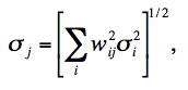 |
(Eq. 11) |
where wij = (rij/σi2) / (∑irij/σi2). Equation 11 assumes the detector-pixel measurement errors (in the Di) are uncorrelated. Note that this represents the co-add flux uncertainty based on priors. With Nf overlapping input frames and assuming σi = constant throughout, it's not difficult to show that Eq. 11 scales as: σj ~ σi / √(NfPj), where Pj = 1 / ∑irij2 is a characteristic of the detector's PRF, usually referred to as the effective number of "noise pixels". This scaling also assumes that the PRF is isoplanatic (has fixed shape over the focal plane) so that Pj = constant. Furthermore, the depth-of-coverage at co-add pixel j is given by the sum of all overlapping PRF contributions at that location: Nj = ∑irij. This effectively indicates how many times a point on the sky was visited by the PRF of a "good" detector pixel i, i.e., not rejected due to prior-masking. If no input pixels were masked, this reduces to the number of frame overlaps, Nf.
Figure 10 shows a schematic of a detector PRF mapped onto the co-add output grid. The PRF boundary is shown as the dashed circle and is centered on the detector pixel. To ensure accurate mapping of PRF pixels and interpolation onto the co-add grid, a finer cell-grid composed of "pixel cells" is set up internally. The cell size can be selected according to the accuracy to which the PRF can be positioned. The PRF is subject to thermal fluctuations in the optical system as well as pointing errors if multiple frames are being combined. Therefore, it did not make sense to have a cell-grid finer than the measured positional accuracy of the PRF. Note that even though the WISE PRFs are non-isoplanatic (systematically vary in shape over each focal plane), the PRF and cell pixel sizes are coarse enough to smooth over such spatial variations.
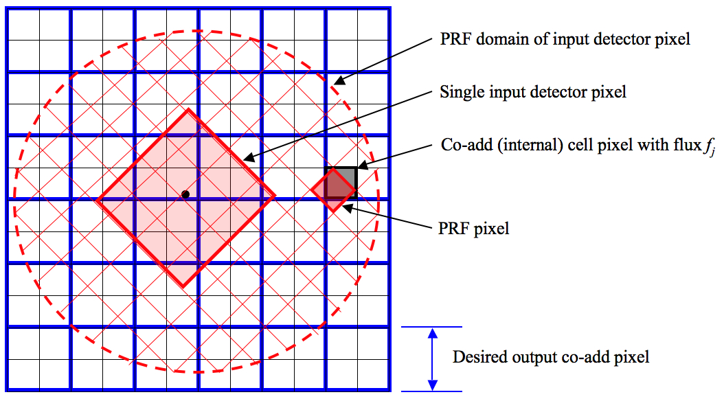 |
| Figure 10 - Schematic of PRF interpolation for a single input pixel. |
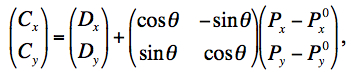
The PRF pixels are mapped onto the cell-grid frame by first projecting the center of the detector pixel with a correction for distortion, and then using a linear transformation to determine the positions of the PRF pixels in the cell-grid:
 |
(Eq. 12) |
where (Px, Py) is a PRF pixel coordinate, (P0x, P0y) center-pixel coordinates of the PRF, (Dx, Dy) are the detector pixel coordinates in the cell-grid frame, and the outputs (Cx, Cy) are the coordinates of the PRF pixel in the cell-grid frame. θ is the rotation of the input detector image (hence PRF) with respect to the co-add (footprint) frame. We have set θ to zero owing to the fact that the WISE PRFs are highly axisymmetric at the coarsely sampled PRF pixel scale used for co-addition. There is negligible difference in co-add products if detector PRF-to-footprint rotation is allowed for.
The value of a PRF-weighted detector pixel flux rijDi in a co-add cell pixel j (see Figure 10) is then computed using nearest-neighbor interpolation. This entails rounding the output coordinates (Cx, Cy) to the the nearest integer cell pixel. An exact overlap-area weighting method for mapping PRF pixels to cell grid pixels was first used, but was computationally slow. After all input pixels (with their PRFs) have been mapped, the internal co-add cells are down-sampled to the desired output co-add pixel sizes (blue grid in Figure 10).
There are two reasons why we used the PRF interpolation method. First, it reduces the impact of masked (missing) input pixels if the data are well sampled, even close to Nyquist. This is because the PRF tails of neighboring "good" pixels can overlap and stretch into the bad pixel locations to effectively give a non-zero coverage and signal there (see schematic in Figure 1 of section II.3.d.). Second, Eqs 10 and 11 can be used to define a linear matched filter optimized for point source detection by deriving a SNR map (ratio of background subtracted intensity image/uncertainty map). This effectively represents a cross-covariance of a point source template (the PRF) with the input data. It leads to smoothing of the high-frequency noise without affecting the point source signal sought. In other words, the SNR per pixel constructed from Atlas Image products is maximized for detecting point source peaks. The inclusion of inverse-variance weighting further ensures that the SNR is maximized since it implies the co-added fluxes will be maximum likelihood estimates for normally distributed data. This methodology is used in the source-detection step of the multiframe pipeline.
Two consequences of PRF-interpolation are that first, it leads to smoothing of the input data in the co-add grid (see cautionary note I.4.c.xi). This may be a good thing since it mitigates pixel-noise, however, cosmic rays can masquerade as point sources (albeit with narrower width) if not properly masked. For an input Gaussian profile for example, the effective width will increase by a factor of ~√2, or the flux per unit solid angle will decrease by a factor of 2 after interpolation, equivalent to convolving the input profile with itself. Second, PRF-interpolation will cause the noise to be spatially correlated in the co-add, typically on scales (correlation lengths) approaching the PRF size. Both the effects of flux smearing and correlated noise must be accounted for in photometric measurements off the co-add. Ignorance of correlated noise will cause photometric uncertainties to be underestimated. Methods on how to account for correlated noise in photometry off the WISE Atlas Images are outlined in section II.3.f.
Last update: 2012 February 20