


Global and local variations in the depth-of-coverage are expected from the nominal survey design (section VI.2). However, there are regions where the depth-of-coverage varies considerably due to the exclusion of "bad" input frames and individual pixels when generating the Image Atlas. This could be due to contamination from the moon, cosmic rays, and/or other outliers (e.g., induced by fast moving objects), or bad quality frames in general. The latter are usually associated with elevated noise or degraded image quality caused by excursions in spacecraft tracking. For details on the frame selection process, see section V.2.c. A general description of the construction of the depth-of-coverage maps and the physical meaning of pixel values therein is given in section II.3.d.
Examples of Atlas Images with low depth-of-coverage are shown in section VI.2.c. An immediate consequence for regions with low depth-of-coverage (covered effectively <~ 6 times) is that the temporal pixel-outlier rejection process becomes unreliable. Even though robust estimators were used in this method, they are still relatively "noisy" when the number of samples in the stack was low. Strictly speaking, no temporal pixel-outlier rejection is performed for depths-of-coverage ≤ 4. This criterion avoided throwing away too many good pixels during the coaddition process, with the caveat of increasing the number of unreliable or spurious detections (cosmic rays, fast moving object trails, and other transients). Note that the Source Catalog selection process explicitly excluded extractions from regions with a depth-of-coverage ≤ 4.
If one were to measure the equatorial (J2000) positions of sources off Atlas Images, e.g., via a flux-weighted centroid or peak-finding algorithm, there could be a systematic difference with the astrometrically calibrated positions from the WISE Source Catalog. The latter was calibrated with respect to 2MASS to an accuracy of <~ 0.4 arcsec over the sky (section VI.4). For reasons not yet understood, the absolute (radial) differences between Atlas Image-derived source peaks and "true" astrometric positions vary with location on the sky and are typically <~ 0.25 arcsec for bands 1 and 2, and <~ 1.2 arcsec for bands 3 and 4 (90th percentile upper limits). A procedure to correct the Atlas Image-derived source positions and/or image WCS in general (if significant biases exist) is given in section II.3.g.
Pixel units in the Atlas Images (and single-exposure images) are not calibrated in terms of absolute surface brightness. Their units are digital numbers (DN). The images are designed for photometric measurements relative to a local background using the photometric Zero Point Magnitude (MAGZP) provided in their FITS headers. Section II.3.f describes how the Atlas Image DN values (and measurements derived therefrom in DN) can be converted to absolute flux units.
One of the first steps in the Atlas Image generation pipeline is background level matching of the single-exposure frames. Since WISE had no requirements for measuring the absolute intensity of the background, we adopted a simple, fast, locally self-consistent method. Only the single exposure frames touching an individual Atlas Image tile (independent of all those touching neighboring tiles) were matched with respect to each other. Two caveats of this method are:
The Anomaly Gallery contains examples of the artifacts commonly encountered in Atlas Images. Overall, these fall in two broad categories, with much overlap between the two:
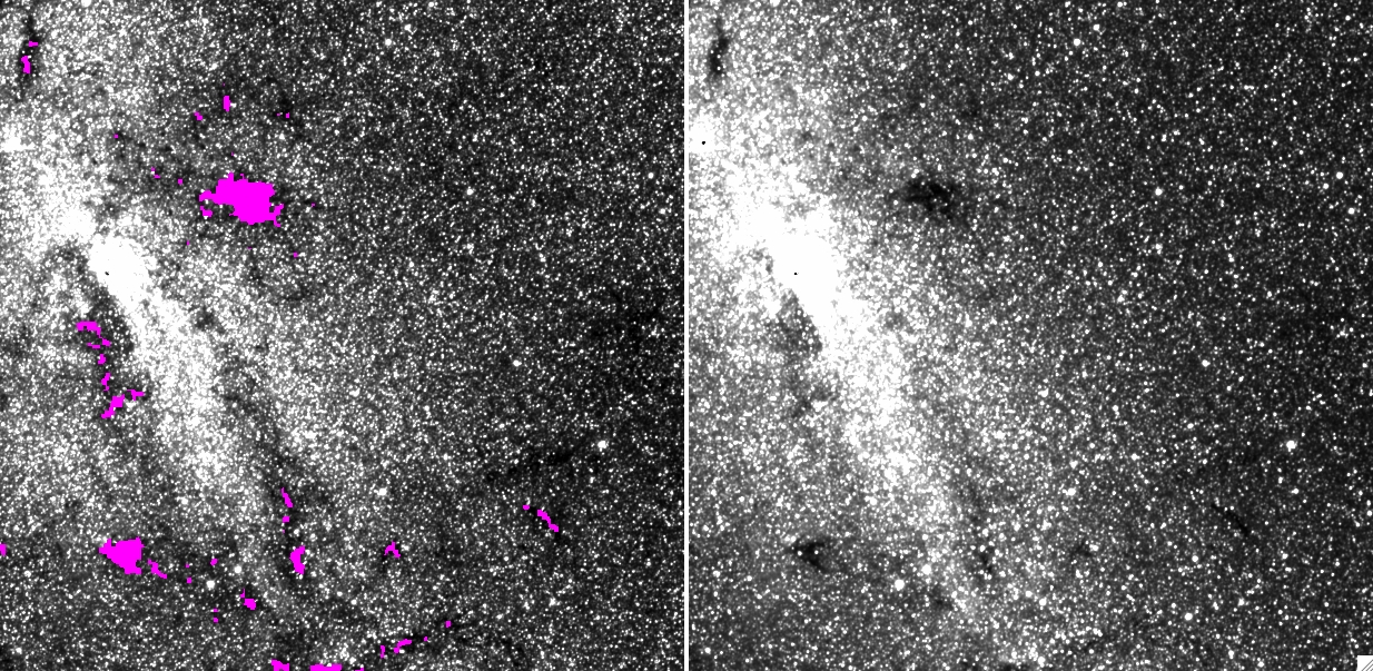
Saturated pixels are masked in the single exposure frames and omitted when constructing the Atlas Images. For bright regions and sources exceeding the saturation limits, pixels in the Atlas Image intensity and uncertainty maps will be associated with NaN (Not-a-Number) values. The corresponding depth-of-coverage map will have zero coverage in these regions. These "holes" are typically seen at the location of the peak-emission of sources. An example is shown here.
The automatic saturation tagging that occurred on board the WISE spacecraft worked rather well, however, there were times when it was not reliable. This occurred intermittently when the counts were at the highest end of the dynamic range in any band. Hence, there are instances in regions of very bright emission, including the cores of very bright sources where saturated frame pixels (with anomalous values) were included when constructing the Atlas Images. The values of these pixels are generally low relative to that expected for the region. An example is shown in Figure 1 and it is generally seen in all bands. Given that the single exposures were also affected and used for simultaneous PSF-fit photometry, the impact on the catalog photometry is described in section I.4.b.
In regions with complex emission or a fast spatially-varying
background (e.g., parts of the galactic plane),
pixels may be erroneously tagged as
outliers across a stack of input frames by the
pixel-outlier rejection step.
This results in sporadic holes (NaNs) in the Atlas Images,
particularly in bands W1 and W2 (e.g., Figure 1).
This is caused by the large variance in the background levels
within frame-overlap regions.
For details, see the last paragraph in
section IV.4.f.3.
The number of tagged outliers is further inflated by the
outlier-expansion step (intended for moving
object mitigation) since this is triggered when the spatial density of outliers
exceeds some threshold. One set of outlier detection/expansion
parameters were used for the entire sky for each band.
Given the heterogeneous nature of the survey, there's no
guarantee this parameter set produced consistent results throughout.
 |
 |
| Figure 1 - Atlas Image cutouts near the galactic center: bands W1, W2, W3, W4 - top left, top right, bottom left, and bottom right respectively. Magenta regions represent NaN'd (zero-coverage) regions. W1 shows an example of the outlier-overtagging anomaly (NaNs at otherwise genuine depressions in the emission); W3 and W4 show examples of the impact of including frame pixels which were not masked for saturation (dark depressions meshed with NaN'd regions properly masked for saturation). |
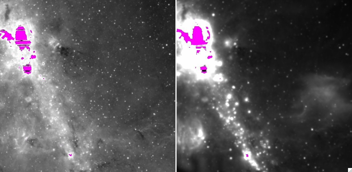
In regions with very-bright emission, W3 and W4 Atlas Images often show
banding patterns with depressed flux. The regions need not be saturated
or close to saturation. This effect is due to inadvertently unmasked
pixel rows at the top and bottom edges of the input W3 and W4
single-exposure frames that have a relatively low
responsivity. These low-response rows were not completely captured in the
static flat-field calibration products to enable their removal since their
responsivity was slightly transient.
Given that the low-response pixel rows
have a multiplicative effect on the signal
that falls on them, higher signals will suffer a
proportionally greater loss in their output counts. These
anomalously low counts fall below
the detector saturation thresholds and therefore remain unmasked.
This banding effect is seen in the bright regions
of the W3 and W4 Atlas Image-cutouts shown in Figures 1 and 2.
Note that the flux along a "band" could be depressed by as much as 12%
over the entire length of the band spanning an Atlas Image.
Therefore, all sources or emission intercepting such bands are likely
to have a biased flux.
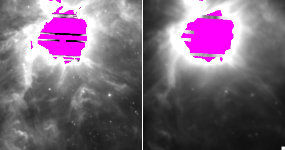 |
| Figure 2 - Atlas Image cutouts showing the core of the Orion Nebula, left: W3; right: W4. Magenta regions represent NaN'd (zero-coverage) regions due to saturation in all the input frames at that location. See section I.4.c.x. for details. |
The effective size of the PSF in an Atlas Image is not the same as that inferred from the single-exposure frames. For the latter, the azimuthally-averaged FWHM of a point source profile is ≈ 5.8″, 6.4″, 6.7″, and 11.8″ for bands W1, W2, W3, and W4 respectively (e.g., see Table 1 in section IV.4.c.iii.1). For Atlas Image (co-adds) however, the FWHM of a point source profile is ≈ √2 times larger than the native (single-exposure) values, or ≈ 8.3″, 9.1″, 9.5″, and 16.8″ in W1, W2, W3, and W4 respectively (however, see caveat below). This additional smoothing arises from use of the native PSF as an interpolation kernel during the co-addition process (for details, see section IV.4.f.vii). This includes the small inevitable amount of smoothing from mapping onto a new grid with finite-sized pixels. The PSF-interpolation makes the Atlas Images also serve as match-filtered products optimized for detecting sources in the pipeline (for details, see section IV.4.b).
The Atlas Image PSF FWHMs quoted above are global ballpark measures and not representative of any one Atlas Image. A "highly-homogenised" set of Atlas Image PSFs is provided in section IV.4.c.viii. These were created from Atlas Images at high ecliptic latitudes where the high depth-of-coverage and large spread in single-exposure rotations acted to circularize the PSF. Owing to the asymmetric nature of the native PSFs (even after co-addition for low-to-moderate depths-of-coverage), we recommended you derive the PSF for your Atlas Image of interest. To obtain an accurate PSF, you may need to combine measurements from multiple Atlas Images with similar depths-of-coverage and input single-exposure geometries.
Last update: 2012 May 15