IV. WISE Data Processing

4. Pipeline Science Modules

a. Single Frame Exposure Instrumental Calibration (ICal)

Contents

i. Overview

The purpose of instrumental calibration (ICal) is to read in a raw (Level-0 or L0) single exposure frame and correct it for instrumental signatures, e.g., dark current, non-uniform responsivity, non-linearity, and other detector-induced electronic signatures. Optical artifacts and signatures induced by telescope optics, e.g., ghosts, glints, global FOV distortion, PSF non-isoplanicity, including image persistence (latents) are not discussed here. These are covered in detail under the ARTID processing system. ICal also initiates pixel uncertainties for a frame using a noise model. These uncertainties are propagated and updating downstream as calibrations are applied. A bit-mask image is also initiated per frame and updated. This stores the status of processing on each pixel as well as prior knowledge of bad hardware pixels. The intent here is to summarize processing algorithms, how calibrations were made, and their overall performance.

The calibrations are band dependent and differ considerably between the HgCdTe arrays (serving W1, W2 at 3.4, 4.6μm respectively) and Si:As arrays (serving W3, W4 at 12.1, 22.2μm respectively). A description of the payload and detectors is given in section III.2. Details on pre-flight characterization and specific detector properties are given in Mainzer et al. 2008. It's important to note that the pre-flight (ground) calibrations differed significantly from those made using on-orbit data. This could be due to the different environment and/or electronics used in ground testing.

The ICal pipeline generates three (level-1b or L1b) FITS image products per band: the main calibrated intensity frame, accompanying uncertainty frame, and mask image. These are generically named: frameID-wBAND-int-1b.fits, frameID-wBAND-unc-1b.fits, and frameID-wBAND-msk-1b.fits respectively.  The uncertainty image contains a 1-sigma error estimate in the intensity signal for every pixel and are used in generating the Atlas Image uncertainty maps. Quality Assurance (QA) metrics and plots are also generated for each frame. For details on frame QA, see section IV.6.a.ii.

The pixel units of a raw input L0 frame are expected to be those as generated by the on-board Digital Electronics Box (DEB). The DEB (Data Number or DN) output is given by Eq. 1. It has the general form: a + b*slopefit, where slopefit is the fitted slope (or rate) to non-destructively read Sample-Up-the-Ramp (SUR) values generated by the Focal-plane Electronics Box (FEB), and a, b are constants. The pixel values in a calibrated intensity frame therefore scale as ∝ slopefit (or the photon accumulation rate), where the bias term a is implicitly removed by the dark subtraction step. A calibration factor (or equivalent photometric zero-point offset) is computed downstream in the WSDS pipeline using photometry relative to a standard star network (see section IV.4.h.ii). This information is stored as the MAGZP keyword in the FITS headers of L1b products, and allows one to convert from DN to absolute flux units (e.g., see Eq. 1 in section IV.4.f.ii).

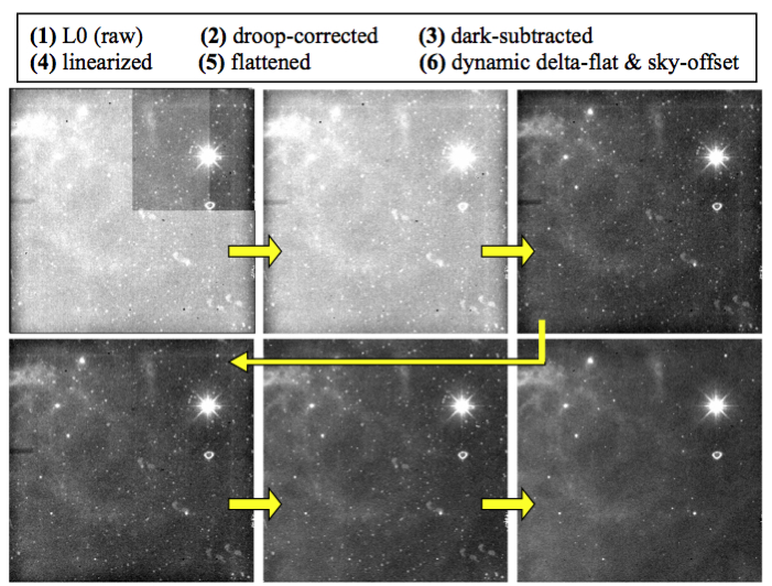
Figure 1 captures the major processing steps in ICal. The cyan/bluish-colored boxes indicate steps generic to all bands. The yellow boxes are specific to W1 and W2 only, while red is specific to W3 and W4. Intermediate frame inputs for offline flatfield creation (compflat) and the dynamic calibration pipeline (dynacal) are shown in green.

Figure 1 - Processing flow in WISE instrumental calibration (ICal) pipeline. Cyan boxes are steps generic to all bands; yellow boxes are specific to W1 & W2; red boxes are specific to W3 & W4; and green boxes show inputs to support calibrations.

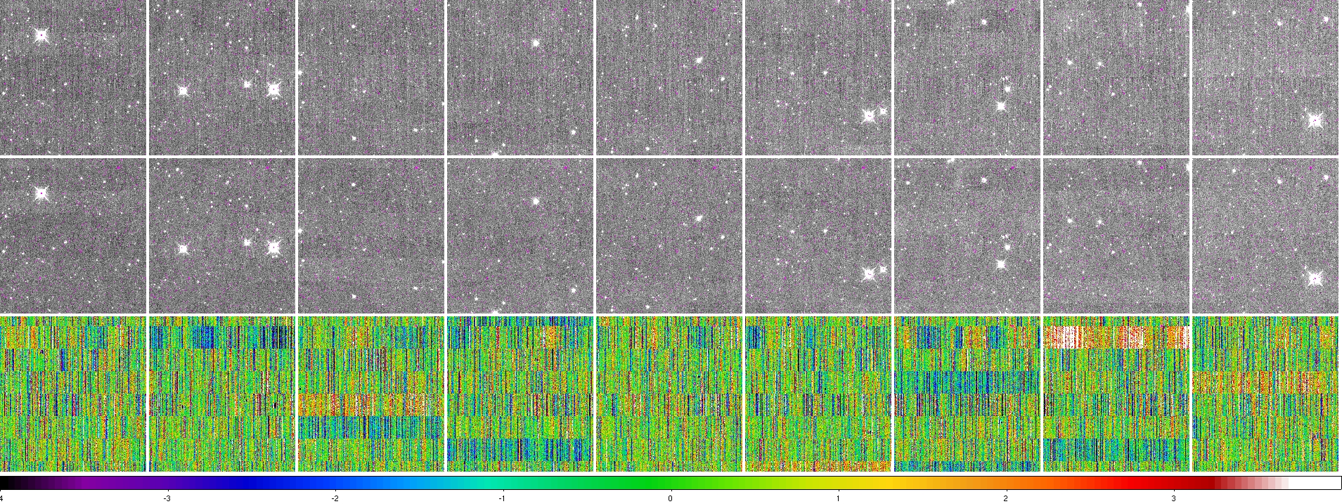
Figure 2 and Figure 3 respectively show examples of W1 and W3 intensity frames processed at various intermediate steps of the ICal pipeline. Results for W2 and W4 are similar. The incremental improvements are more easily noticeable in processing of the Si:As arrays (W3 and W4), in particular in the droop and dynamic calibration steps in Figure 3. The dynamic calibrations have nicely removed the trail of latent footprints along the diagnonal of the frame.

Figure 2 - Images of intermediate primary instrumental calibration steps for W1. Corresponding steps are shown in the box. Stretch is the same for all images. Pink areas in the final L1b frame are NaN'd (bad) pixels. W2 is similar.

Figure 3 - Images of intermediate primary instrumental calibration steps for W3. Corresponding steps are shown in the box. Stretch is the same for all images. Note: the final L1b frame with NaN'd pixels (like the last in Figure 2) is not shown here. W4 is similar.

i.1. Input Calibration Summary

The pertinent detector calibrations are summarized in Table 1. Also shown is the origin of the data used to create the calibration product for each band ("ground", In-Orbit Checkout [IOC], and/or "survey"), and the format, i.e., whether the calibration was created for every frame pixel ("image"), or whether a single number was only possible. Static calibrations made from "survey" observations used science data over the course of the cryogenic mission (~mid January 2010 to ~mid July 2010). Dynamic flat-fields, sky-offsets, and transient bad-pixel masks were made on a per frame basis throughout the mission.

i.2. Bit-Mask Definitions

The frame mask is a 32-bit image product (generic name frameID-wBAND-msk-1b.fits) that stores pixel status information for its corresponding single exposure intensity frame (frameID-wBAND-int-1b.fits). It stores both "static" information on bad-hardware pixels (replicated from the static calibration mask) and dynamic information on which pixels became saturated and transiently bad, and any hiccups/warnings in the application of calibrations during processing. The mask is initialized and updated in the ICal pipeline (see section iii.) and further updated downstream in the outlier detection step of the co-addition pipeline. The primary purpose of the frame mask is to omit bad, saturated, and outlying frame pixels when generating the Image Atlas.

The pixels in the frame mask are represented as 32-bit signed integers (FITS keyword BITPIX = 32) with certain conditions assigned to the individual bits. Useable bits are numbered from zero (the Least Significant Bit [LSB]) to 30. The sign bit, bit 31, is not used. If the bit has the value 1, the condition is in effect. Zero implies that the condition is not in effect. Pixel values in a mask can encode a combination of bits. For coding simplicity and to ensure the majority of bad pixels are tagged (i.e., by using more than one method), no attempt was made to keep the bit assignments mutually exclusive. For example, a mask pixel value of 402653208 encodes bits 3, 4, 27 and 28, i.e., 402653208 = 2³ + 2⁴ + 2²⁷ + 2²⁸, where bits tagged as bit 27 (temporal outlier from frame stacking) could also have been tagged as bit 28 (pixel spike from the single-frame glitch filter).

The conditions assigned to each bit, where available, are defined in Table 2. Note: these definitions only pertain to frame products in the all-sky release.

1. Bits 0 - 7 (the first eight) are replicated from the static 8-bit calibration mask for the respective band (section iii.1.). These bits are static in the sense that they are the same for every frame of a specific band. The remaining bits (8 - 30) are set dynamically on a per-frame basis during processing.
2. Bit 3: low responsivity refers to a pixel which is not quite dead (i.e., relative responsivity below normal). Pixels that are truly dead or have very low responsivity are covered by bit 2.
3. The saturation bits: 10 - 18 are dynamically set on a per-frame basis by keying off specific values in the raw (L0) image data. For details, see section iii.
4. Bit 21: new or transient bad pixels (primarily those that have gone high or low relative to their neighbors for some period) are detected and tagged using dynamic masking in the dynamic calibration pipeline (dynacal).
5. Bit 27: this is a generic condition pertaining to any outlier detected using the temporal frame stacking method as described in section IV.4.f.v. It will tag transients inadvertently missed by other methods, as well as sources that may have moved or varied appreciably between overlapping frames.
6. Bit 28: records "hard-edged" pixel regions and/or spikes detected at the single frame level in ICal (see section ix.). There may be redundancy with outliers detected by the temporal detection method (bit 27).

NaN'ing of bad frame pixels

The frame masks are used at the end of ICal processing to reset pixel values in the final calibrated intensity and uncertainty frame products to NaNs. Only pixels with specific fatal conditions are reset. The fatal conditions in Table 2 for NaN'ing frame pixels in the all-sky release are those defined by any of the following bits: 0, 1, 2, 3, 4, 9, 10, 11, 12, 13, 14, 15, 16, 17, 18. This applies to any band.

ii. Pixel Error Model

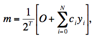
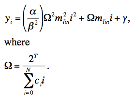
In general, the observed raw signal m per pixel is computed on-board from a linear combination of non-destructively read Samples Up the Ramp (SUR) y_i:

(Eq. 1)

where nominally N = 8; c_i are the SUR weighting coefficients: {0,-7,-5,-3,-1,1,3,5,7} for W1 & W2, and {-4,-3,-2,-1,0,1,2,3,4} for W3 & W4; O is an offset (= 1024 for all bands), and T is the number of LSB truncations, where T = 3, 3, 2, 2 for W1, W2, W3, W4 respectively. The time interval between the sample reads y_i is 1.1 sec. This results in an effective pixel exposure time of 7.7 sec for W1, W2 and 8.8 sec for W3, W4. The shorter exposure time for W1, W2 is due to omission of an erratic first sample (with weight c₀ = 0).

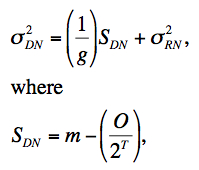
One-sigma uncertainties for each pixel in an input frame are initialized using a simple traditional Poisson + read-noise model. The noise-variance in a pixel signal m (in DN²) can be written:

(Eq. 2)

g is the electronic gain in electrons/DN, and σ²_RN is the read-noise variance in units of DN². The bias term O/2^T as defined above is removed before computing the Poisson noise component. The gain and read-noise terms were determined using on-orbit image data as described in section ii.1. The benefit of deriving these terms empirically is that certain multiplicative factors due to for example spatially correlated noise from pixel cross-talk and correlated noise between reads in the SUR technique (Eq. 1) can be absorbed into the parameter g (which no longer becomes a "true" electronic gain). As shown in section ii.1., we find that this method accurately predicts a posterior estimates of the pixel noise as measured from RMS fluctuations in the background. Also, the reduced χ² metric from PSF-fit photometry to point sources, i.e., effectively the ratio: [variance in fit residuals]/[prior noise-variance propagated from Eq. 2 + other photometric noise terms] is on average ≈ 1. Note that PSF-fit photometry and other relevant noise terms (e.g., source confusion) are described in section IV.4.c.iii. The uncertainty estimated from Eq. 2 was propagated and updated as each calibration was applied, i.e., uncertainties in the calibration products were appropriately RSS'd with the frame-pixel uncertainties at each step of the pipeline.

ii.1. Electronic Gain and Read-Noise Calibration

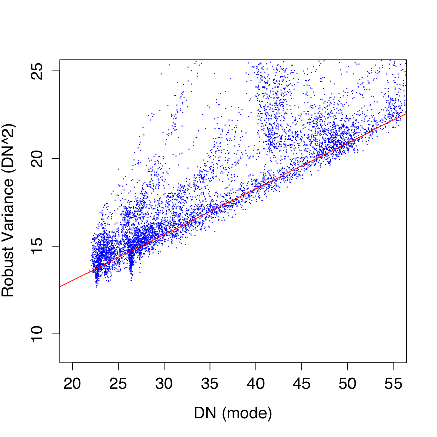
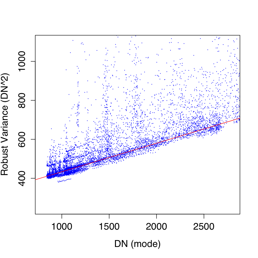
The effective gain and read-noise terms in Eq. 2 were estimated from on-orbit data by first computing robust measures of the spatial pixel variance (σ²_DN) and modal signal (S_DN) in ~7000 instrumentally calibrated frames spanning the full ecliptic latitude range. The robust variance metric used the lower-tail standard deviation from the pixel mode (with low-tail outliers trimmed). The spread in ecliptic latitude provided a varying background signal (and spatial variance) in all bands to allow a fit of Eq. 2 to measurements of σ²_DN versus S_DN. The slope from such a fit is then simply 1/g and the intercept is the read-noise variance σ²_RN, the square root of which is the read-noise sigma sought for.

Even though robust metrics for the measurements were used, they were still affected by the inevitable presence of sources and structure in the background. We therefore performed the fitting of Eq. 2 using a robust linear regression method based on the concept of the M-estimator. Plots of fits to the data are shown in Figure 4 with parameter estimates for g and σ_RN given in columns 2 and 3 of Table 3. Our robust fits more-or-less spanned the lower envelope of the variance distribution at each modal signal level, i.e., that represented by the underlying background.

The above method yielded single estimates of the effective gain and read-noise for all pixels of a band in general. It would have been a tedious task to estimate these parameters for each pixel using the above method (e.g., by measuring instead the temporal stack variance versus signal level for each pixel). We therefore adopted the single gain estimates as listed in Table Table 3 for use in Eq. 2. For the read-noise however, we combined the single fitted values for σ_RN with read-noise maps derived from stacking cover-on dark data during IOC. The modes of these dark/read-noise maps are listed in column 4 of Table 3, and only W1 and W2 were reasonably close to our single parameter estimates. The discrepancy for W3 and W4 is described in note [2] of Table 3. In the end, we rescaled the dark/read-noise maps from IOC by the ratio: [fitted σ_RN]/[mode of IOC RN map] to arrive at read-noise maps for use in the pipeline.

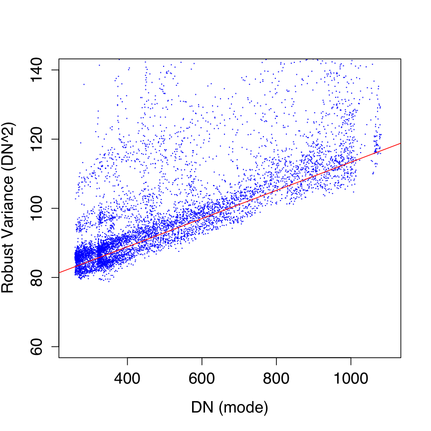Figure 4 - Robust pixel variance versus modal pixel signal for W1, W2, W3, W4 (left - right). Red lines are robust fits of Eq. 2 with best fit parameters in Table 3.

1. Derived from fitting noise model (Eq. 2) to survey data. These values are used in the pipeline.
2. For comparison, these read-noise sigmas were derived by stacking cover-on dark images acquired during IOC, computing a robust RMS (trimmed standard-deviation) of the pixel stacks, then computing the mode of all pixel RMS values. Note that owing to a warm telescope cover after launch, the W3 and W4 arrays were kept in a de-biased state during IOC. Therefore, the absolute W3 and W4 stack-RMS values listed here are not expected to be representative of the true read-noise for these arrays. From a comparison to ground test products, only the relative pixel-to-pixel (spatial) variation in the W3, W4 cover-on RMS images is expected to have meaning.

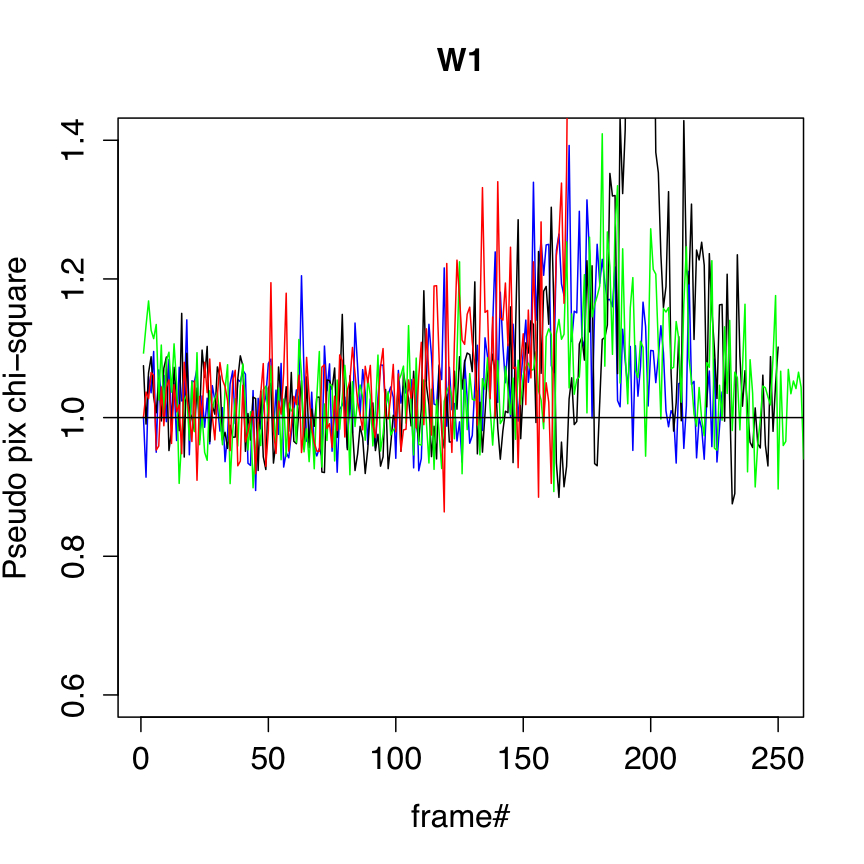
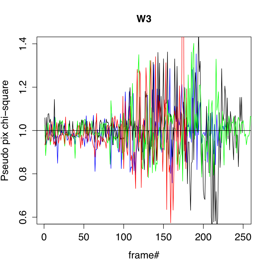
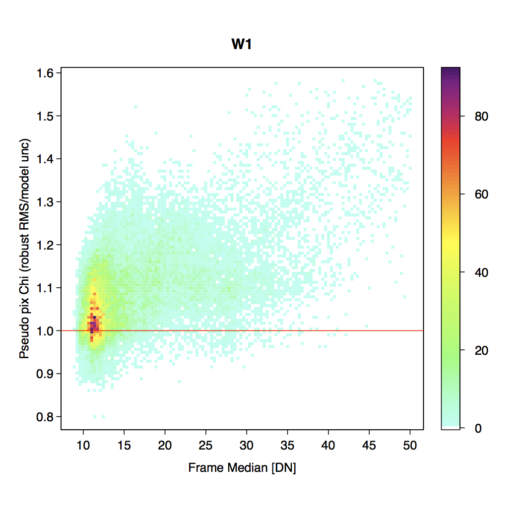
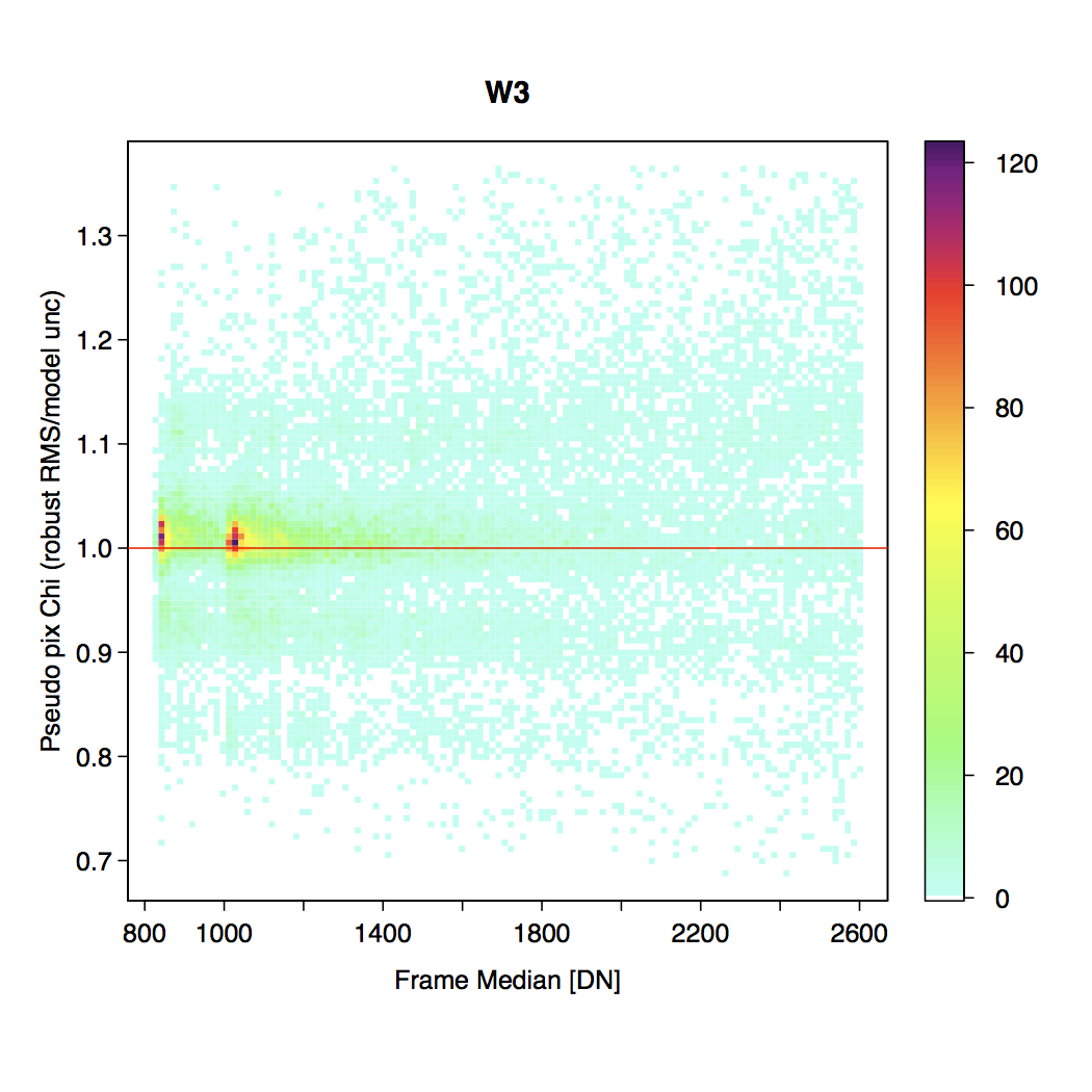
The uncertainty frame products were validated against measurements of the RMS fluctuation about the background in the corresponding intensity frames. We used an automated algorithm to select frame background regions that were approximately spatially uniform and with low to moderately low source-density. A trimmed lower-tail standard deviation from the mode was used as a proxy for the RMS. This measure was divided by the modal pixel uncertainty over the same regions (as estimated and propagated from Eq. 2) to arrive at a pseudo reduced χ² measure per pixel. This measure is shown as a function of frame number for four different survey scans in Figure 5a. These scans came close to the galactic plane with the source density peaking at around frame number 180. Our robust RMS metric was not totally immune to the presence of astrophysical structure and hence exceeded the uncertainty model prediction at these locations. Figure 5b shows density plots of the same ratio versus frame pixel median using ~25,000 frames in total.

Overall, the uncertainty model is seen to track noise fluctuations in the underlying background reasonably well, both in the read-noise limited W1, W2 bands, the quasi-readnoise limited W3 band, and the background-photon dominated W4 band. This holds all over the sky (setting aside contributions from source confusion) and throughout the duration of the cryogenic mission. It is also encouraging that global analyses of PSF-fit photometry to point sources show reduced χ² values of ≈ 1 on average for all bands (section IV.4.c.iii).

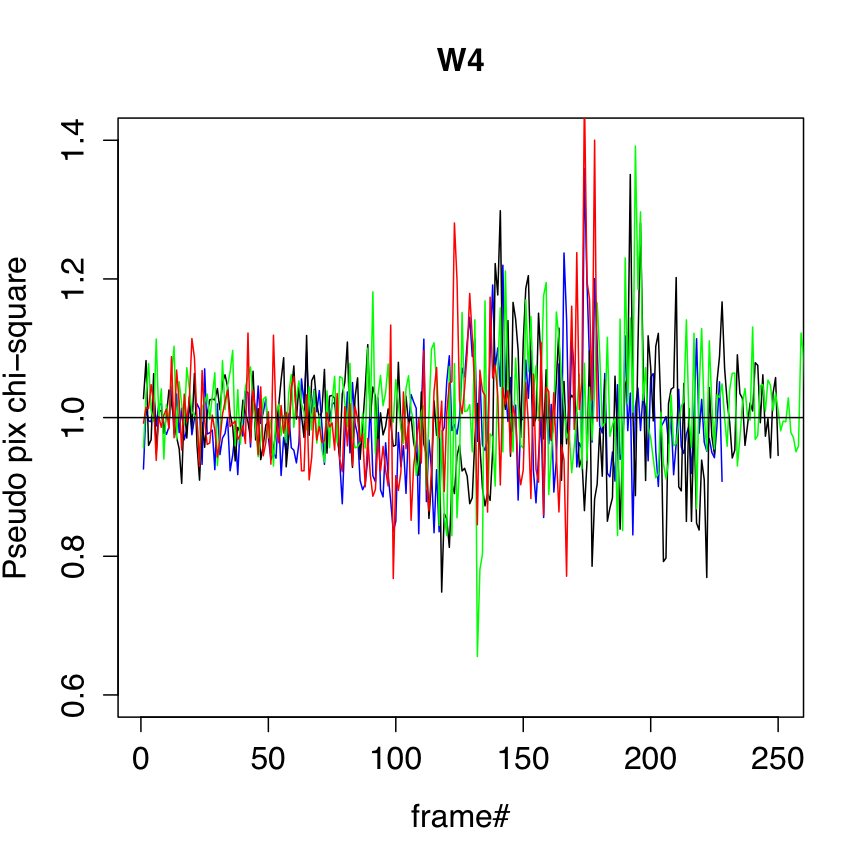Figure 5a - Ratio of "robust pixel RMS/model (modal) pixel uncertainty" versus frame# for four different scans (colored) for W1, W2, W3, W4 (left - right).

Figure 5b - Ratio of "robust pixel RMS/model (modal) pixel uncertainty" versus frame median for ~25,000 frames (per band) shown as color-density plots. Color-coded values are represented by the color bar. Results are given for W1, W2, W3, W4 (left - right).

iii. Frame-mask Initialization and Bad-pixel Masking

The frame-mask product (frameID-wBAND-msk-1b.fits) and bit-definitions therein were described in section i.2. This mask is initialized in the ICal pipeline by first copying all information from the static calibration mask into the first 8 bits of a 32-bit buffer (see Table 2). Next, we set the dynamic bits: 9 - 18 according to specific values in the input raw L0 frame. These were assigned on-board the spacecraft during Sample-Up-the-Ramp (SUR) processing (section ii.). L0 pixel values of 32,752 + n, where n=1...9 are reserved to encode the SUR number where a ramp begins to saturate after A/D conversion. n=1 corresponds to the first sample read and means the entire ramp is saturated. This is usually referred to as "hard" saturation. The L0 values 32,752...32,761 are therefore assigned to the 9 saturation bits: 10...18 respectively. As a detail, hard saturation for W1 and W2 will occur at n=2 since the first sample for these bands is unreliable and excluded from on-board SUR processing (therefore, bit 10 is never set for W1,W2). Hard saturation for W3 and W4 will occur at n=1. Furthermore, the special L0 value 32,767 is assigned to bit 9 and usually means that the on-board SUR processing yielded a negative slope measurement, e.g., due to a noise spike or glitch in the ramp.

Occurence of missed (unmasked) saturated pixels

In general, the automatic saturated tagging that occurred on board the spacecraft worked rather well, however, there were times when it was not reliable. This occurred intermittently when the counts were at the high end of the dynamic range in any band. Hence, there are instances in regions of very bright emission, including the cores of very bright sources where saturated frame pixels (with anomalous values) were not masked as saturated. Instead, the values of these pixels are generally much lower (and sometimes negative) relative to that expected for the region. The impact on photometric measurements in the Source Catalog is described in section I.4.b.

iii.1. Prior Masking of Bad Hardware Pixels

Bit values in the frame mask products were defined in Table 2, with the first 8 bits copied from the static bad pixel calibration masks. The static bad pixel masks represent the population of pixels permanently masked from processing because they have the potential to compromise photometric accuracy and precision. Criteria for the rejection of pixels relate to the level at which any one of these phenomena has the potential to add to the uncertainty of or bias the flux for an extracted point source. Inputs to static bad pixel mask generation included:

• dark images generated from both true dark data acquired during the post-launch period where the cover was still on the telescope for W1 and W2 and extrapolation of the dark frame intercept from flat field analysis of on-sky frames for W3 and W4.
• flat-field images and the associated uncertainty maps constructed from combination of large numbers of on-sky frames in all four bands.
• "readnoise" images produced by evaluating the RMS uncertainty for a series of un-illuminated frames. For W1 and W2 these frames were acquired post-launch but prior to the ejection of the telescope cover. For W3 and W4 the cover was too warm to permit the measurement of true dark frames after launch. Ground test data in which the cover was cooled, and thus dark, provided the noise data for static mask generation for W3 and W4. Note that W3, W4 read-noise products derived for the error model (section "readnoise" images) were not used for mask generation.
• (non)-linearity calibration products from characterization of ground test data.

Conditions that trigger the identification of a static bad pixel include:

• non-responsive pixels
• excessively high dark current
• non-linearity
• excessive noise
• underresponsive or excessively responsive pixels.
• excessive noise in flat field determination

Many of these conditions are inter-related. For example, pixels with significant dark current exhibit excessive Poisson noise in the fixed WISE exposure time and can be a readily rejected based on their noise behavior. Each of these conditions was evaluated independently from the others so that pixels could be rejected for multiple conditions and combined into a final static bad pixel mask for each band that encoded all of the rejection thresholds violated by any given pixel.

Bad pixel rejection criteria

Responsivity:
Flat fielding corrects for relative pixel response, even if that response is significantly outside the median response of the array. The static bad pixels masks reject pixels which lie abnormally outside the distribution of pixel responsivity for a given array. These conditions are tagged as bits 2, 3, and 4 in the masks (see Table 2).

Dark current and excessive noise:
Pixels can be flagged as noisy because of intrinsic instability or due to Poisson noise from excessive dark current. Pixels were identified for static masking due to excessive noise if the RMS noise in that pixel was three times the median RMS noise for pixels across the array for W1 and W2 and two times the RMS noise in W3 and W4. Pixels with three times the array RMS would inflate the uncertainty of a faint source by 10% if the source extraction footprint extends over 10 pixels. The static bad pixel masks also account for pixels with abnormally low RMS noise - those which lie below the main distribution - as was the case for responsivity masking. These conditions are tagged as bits 0 and 1 in the masks (see Table 2).

Flat-field uncertainty:
Flat-field maps were derived from on-sky data as described in section vii. The resulting uncertainty maps for these flat-fields were used to identify statically masked pixels. Thresholds of 2% and 1% uncertainty in the flat field were used from W1/W2 and W3/W4 respectively. For lack of availability of additional bits, these conditions were also tagged as bits 0 and 1 in the masks (see Table 2).

Table 4 provides the responsivity, RMS-noise, and flat-uncertainty thresholds for all bands. Also listed (last column) is the percentage of pixels masked using the criteria listed. This percentage excludes those masked for bad (non)-linearity and the ancillary conditions described below. Furthermore, these statistics only pertain to the active region of each array (1016² pixels for W1, W2, W3, and 508² pixels for W4).

Linearity:
Pixels with a bad (non)-linearity calibration were also included in the static masks (not shown in Table 4). Here, those pixels whose non-linearity estimates were abnormally high, highly uncertain, and/or unreliable as determined from a bad fit to their Sample-Up-the-Ramp (SUR) data were tagged as bit 6 in the masks (Table 2). The thresholds for each band were picked by identifying outlying populations in pixel histograms of the non-linearity coefficient, S/N ratios of their estimates (typically < 2.0), and χ² values falling above or below several times the standard-deviation expected for the number of degrees-of-freedom of a specific fit.

Ancillary:
Two other static bad-pixel conditions listed in Table 2 are bit 5: "saturated anywhere in ramp" and bit 7: "broken pixel or negative SUR". These occured in the input frame data used to generate the calibration products and refer to respectively instances where a hardware pixel was always excessively hot (effectively saturated) or behaving erratically in on-board SUR processing (see section iii.).

In closing, only a subset of the static bad-pixel conditions were used to "NaN-out" pixels in the level-1b intensity and uncertainty frame products. All conditions used for NaN'ing were summarized at the end of section i.2. The static bad-pixel conditions considered fatal enough for NaN'ing are those defined by bits 0, 1, 2, 3, OR, 4 in Table 2, with threshold information summarized in Table 4. As mentioned above, these bits are not mutually exclusive, i.e., more than one of condition could apply to the same pixel. Those static conditions not used for NaN'ing merely serve as a warning.

iv. Band 3 and 4 Droop Correction

Droop is a signature of the W3 and W4 arrays and manifests itself in two forms: (i) intra-quadrant splitting, usually bisecting a saturated source or region, and (ii) global quadrant-to-quadrant (Q-to-Q) effects leading to a depression of one or more quadrants followed by an increase (or rebound) in the quadrant signals in subsequent frames. During the rebound phase, the quadrants also become unstable at the location of bad-pixel clusters and the banding/split structure seen in the dark becomes apparent, lasting for 10-20 frames. These residual bands (in excess of those seen in the static dark calibration) are also referred to as "stationary splits" and were corrected using the same algorithm designed for intra-quadrant droop-splits. All forms of droop have been confirmed to be additive in nature and were corrected using relative in-frame offsets. There is also a final (optional) refinement step for cases where a global Q-to-Q correction could not be computed. We describe the algorithms (in order of execution) in sections iv.1, iv.2, and iv.3. Figure 1 (red boxes) shows the location of these steps in the pipeline flow. Section iv.4 summarizes anomalies and liens from the droop correction.

iv.1. Intra-Quadrant Split-Droop

Here are the steps for correcting this flavor of droop.

1. We start with the raw L0 frame and create an internal regularized split-detection image. This image is made by subtracting the static dark, dividing by the static responsivity map, and replacing bad pixels (using the static bad-pixel mask) with a median of the respective quadrants. The latter is needed since the bad pixels are usually represented as saturated/high values in the input frame and these interfere when trying to search for droop-related splits across real saturated sources downstream. This temporary working frame stored in memory and only used for detecting candidate splits and computing corrections for further dissemination. Actual corrections are applied to the input L0 frame for propagation downstream, as described below. The dark and responsivity corrections are needed because first, the strong edge vignetting in a L0 frame makes the computation of offset corrections close to a frame edge unreliable, and second, the banding-related split corrections are intended to be residual corrections on top of the static dark that is subtracted in processing further downstream. If we did not subtract the dark, we run the risk of removing the entire "static" banding structure using the split corrections, and will need to be replaced (in some cumbersome way) before the final dark is subtracted.


2. We then search for candidate splits in each quadrant. We first collapse the columns of each quadrant (or take a cut across them) by computing quantiles corresponding to some fraction falow (= 0.1) in the low-tail pixel distribution of each column. We choose to work with quantiles in the low-tail of the histogram because they are less biased by the presence of bright extended structure and sources. I.e., such measures will be closer to the underlying background. W3 and W4 are background dominated for the most part, but occasionally, bright extended structure can occur. A median is not as robust against such structure and more likely to overestimate the droop-offset correction. An example comparing the median and quantile differences across a droop-induced split is shown in Figure 6. The real offset appears to be closer to the 10%-tile (0.1 quantile) difference of ~7 DN, and not the much larger median difference of ~54 DN.


3. Given the 1-D vector of column-collapsed quantile values from step 2 for a quadrant, we computed its first derivative (i.e., the vector of first-differenced pairwise values in the increasing x-direction). This derivative vector was thresholded using an input parameter (splithres) to find the locations of all candidate splits. Only those splits which intercepted at least one saturated pixel (section iii.) were retained. These were the "droop-induced" splits. Splits associated with residual banding were retained by comparing the candidate split list with known stationary banding-split locations. The idea here was to be complete in the split detection process by setting splithres to be relatively low (e.g., 4 DN).


4. For a candidate split, the lower-quantile values in strips of width 7 pixels on either side of the split at a distance of 2 pixels from the split were computed. These strips contained more pixels than the single columns used for the initial detection in step 3 and therefore were more reliable at filtering spurious splits. For a given split, the quantile difference of its adjacent strips was then thresholded against a second (but higher) threshold parameter, postsplithres, with magnitude 10 DN. This determined whether the split-step was significant and worth correcting.


5. If a split survived the post-thresholding in step 4, the quantile difference in adjacent strips was then used as the offset correction. This was applied to all active and reference pixels of a quadrant on only the left side of the split in the original L0 frame. Note that it didn't matter which side was corrected. The reference pixels were corrected for self-consistency since they were used to correct the global inter-quadrant droop effect (see below). Note that only pixel columns at distances > 2 pixels from the split were corrected since the split transition region was not necessarily a sharp step. The transition region is treated next.


6. Finally, we corrected the split transition columns which spanned a width of 5 pixels (2 pixels on either side + the split column). For these columns, we use the original column quantile vector from step 2. For each column, offset corrections were computed using the low-tail single column quantiles and the quantile of the strip on the uncorrected side of the split. The goal was to equalize levels in the split transition region with other regions in the quadrant.


7. If there was more than one split in the quadrant, we iterated steps 4, 5, and 6 until all splits and transitions were corrected. To ensure this, the internal working temporary frame was self-consistently updated following each correction. The split corrections were applied to the input L0 frame (to both active and reference pixels) for propagation downstream.

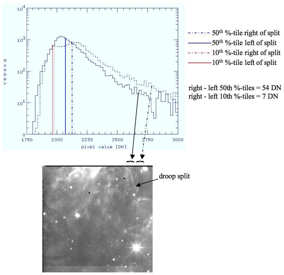Figure 6 - Example of a droop-related split in a quadrant of a W3 frame. This compares the median and lower 10%-tile estimates in the histogram of pixel values in narrow strips on either side of the split.

iv.2. Global Inter-Quadrant Droop

Following the intra-quadrant split corrections, quadrant-to-quadrant (Q-to-Q) relative offsets were then computed and applied to equalize levels over the whole frame. This step exclusively used the reference pixels where possible (which may have been updated by the split correction step above). The correction was computed for each separate quadrant by first computing the median of all its good reference pixels, where "good" meant pixel values < 32,767 (32,767 being the specially encoded L0 pixel value indicating a bad on-board estimate for the pixel signal - see section iii.). This median was only computed if the fraction of good pixels in a reference region was > 0.9.

The median reference-pixel signal for each quadrant was then differenced with its long-term median signal to compute a relative offset correction. These long-run baselines (one for each quadrant in W3 and W4) were calibration inputs. These baselines were seen to be stable over long periods and appeared to represent the natural levels that the reference pixels returned to after a droop and/or rebound event (see Figure 7). The relative corrections were then applied to the active pixels of each respective quadrant. This brought them in line with what one would have observed if no droop or rebound event occurred.

If the fraction of good reference pixels was <= 0.9 for any quadrant, no correction was applied to the active pixels. Instead, a flag was set and propagated downstream to the optional droop-refinement step (see below).

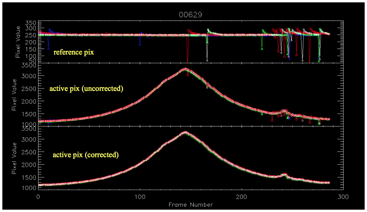Figure 7 - Trend of reference pixel medians (top), corresponding active pixel medians before the Q-to-Q correction (middle), and after correction bottom) for all frames in a scan.

iv.3. Final Droop Refinement

If a global correction using reference pixels alone (section iv.2.) could not be computed for a quadrant, e.g., because there were an insufficient number of good reference pixels, we attempted to compute an offset using the active pixels in neighboring quadrants where a droop-correction was possible. In order to minimize biases from quadrant-dependent instrumental residuals, this step was performed after all instrumental calibrations were applied.  

We first computed lower-tail quantile values in strips of width 50 pixels for W3 and 25 pixels for W4 running up and down the center the frame. Figure 8 shows an example of a correction for quadrant Q1. The correction for this quadrant used the strips colored solid red. If a Q-to-Q droop correction using reference pixels alone was possible for Q2, the offset correction for Q1 was obtained from the quantile difference: quant(Q2) - quant(Q1). This correction was added to all the active pixels of Q1. If a correction was not possible for Q2, we looked at the bottom quadrant, Q4, and used the active pixels in its strip to compute the offset correction for Q1, i.e., quant(Q4) - quant(Q1). The same procedure was used for the other quadrants that failed to be corrected for global Q-to-Q droop (section iv.2.). E.g., for Q3, the correction sought for was first quant(Q4) - quant(Q3), but if Q3 was not initially corrected for Q-to-Q droop, we tried using quant(Q2) - quant(Q3) instead.

If no correction was possible after two attempts at using the neighboring "good" quadrants, we gave up and left it at that. Note that we avoided using strips aligned in the horizontal direction (above/below the quadrants) due to the possibility of badly corrected splits, either from droop or residual banding. This would have biased the active-pixel corrections.

Figure 8 - Schematic for final droop refinement if the reference pixel method for correcting Q-to-Q droop (section iv.2.) for any quadrant could not be used.

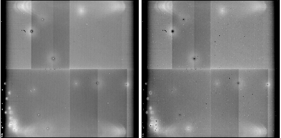
Figure 9 shows a collection of raw (level-0) W3 frames containing "drooped" and droop-induced split quadrants. The calibrated and droop-corrected (level-1b) frames are shown on the right.

Figure 9 - Left: Raw (level-0) W3 frames and Right: same frames after droop corrections and other calibrations were applied. Pink regions are NaN'd bad pixels.

iv.4. Droop correction Anomalies and Liens

As mentioned in the cautionary notes section (I.4.d), droop corrections were not always accurate. Residuals are sometimes seen in all-sky-release W3 and W4 single exposure products. There are two anomalies one should be aware of.

1. Residual signal along columns bisecting bright sources (usually with a saturated core) are sometimes seen. An example is shown in the top right frame of Figure 9 after the correction was applied. This is due to an erroneous column-per-column correction across the split-transition region. Here, the gradient and size of the transition region varied in an unpredictable way.


2. The global quadrant-droop effect sometimes induces curvature in the background level of a quadrant. Its occurrence is unpredictable and unfortunately, it is most often seen when scanning over the Cat's Eye Nebula near the North Ecliptic Pole (NEP), i.e., in the WISE Touchsone Field. Fortunately, this curvature is mitigated in co-adds (Atlas Image products) made over the NEP where frame rotation (due to the intersecting survey scans) helps homogenise the background residuals.

v. Dark Calibration

W1 and W2 darks were generated by stacking ~46,000 cover-on (dark) frames acquired during the In-Orbit Checkout (IOC) period. The stacking used a trimmed averaging method. The dark levels in the calibrations are generally below 1 DN and the 1-σ uncertainty per pixel was of order 0.013 DN for both bands. Figures 10 and 11 compare the flight-derived (IOC) dark calibrations (right) with those derived several months earlier on the ground (left), for W1 and W2 respectively. The major difference is an increase in the number of bad pixels in flight, by ~60% in both bands. This degradation is expected to be due to repeated thermal cyclying of the arrays during testing prior to flight. Nonetheless, the fraction of bad pixels in the W1, W2 arrays was still relatively low and under ~2% (see section iii.1. for a summary of bad pixel statistics).

Figure 10 - Dark calibration images for W1. Left: from laboratory (MIC2 testing); Right: from cover-on flight data. Pixel signals are at same stretch.

Figure 11 - Dark calibration images for W2. Left: from laboratory (MIC2 testing); Right: from cover-on flight data. Pixel signals are at same stretch.

Band 3 and 4 darks

Unlike W1 and W2, the cover was too warm to permit the measurement of dark images for W3 and W4 during IOC. The W3 and W4 arrays were de-biased to minimize degradation during this period. The ground darks were unsuitable for all-sky processing since the on-orbit frames exhibited residual bias structure after the calibrations were applied. This could be due to the different electronics used in ground testing and in flight. We therefore proceeded to estimate darks using illuminated frames from the regular survey. The procedure used ancillary products generated from the responsivity (flatfield) calibration step (section vii.). This is outlined below.

First, we assumed a simple model for the signal observed in detector pixel i:

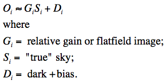(Eq. 3)

A proxy for the "true" sky signal S_i is taken to be the median raw-frame (L0) signal over all array pixels minus some (unknown) absolute dark level D_L, i.e.,

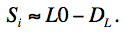(Eq. 4)

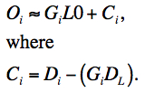
The observation model in Eq. 3 then becomes:

(Eq. 5)

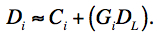
The flat (slope) G_i and intercept C_i were initially estimated by fitting the first line of Eq. 5 to each L0 pixel using the change in the zodiacal background as determined by the median L0 level. This was provided by the responsivity (flatfield) calibration step described in section vii. The dark signal per-pixel was then derived from:

(Eq. 6)

We assumed values of the absolute dark level D_L from ground testing. Regardless of the absolute level, what's important here is that the underlying dark variation (and banding structure) was captured.

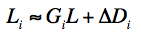
The above method was initially used to derive provisional darks for use in initial processing. However, when more survey data became available, a new set calibrations were generated to support processing for the all-sky release. In this new round, the flatfield products were not generated using L0 frames as inputs, as above, but were generated from prior dark-subtracted and linearized frames. Therefore, instead of fitting to background variations in L0 frames directly, we fitted to the linearized pixels L_i versus their median level L. The latter then became a proxy for the change in overall sky signal S_i ~ L, similar to Eq. 3:

(Eq. 7)

Given the input data had been dark-subtracted using the old (provisional) dark, the intercept ΔD_i from this new fit was the correction needed to derive the new dark from the old (provisional) dark:

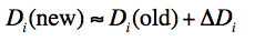(Eq. 8)

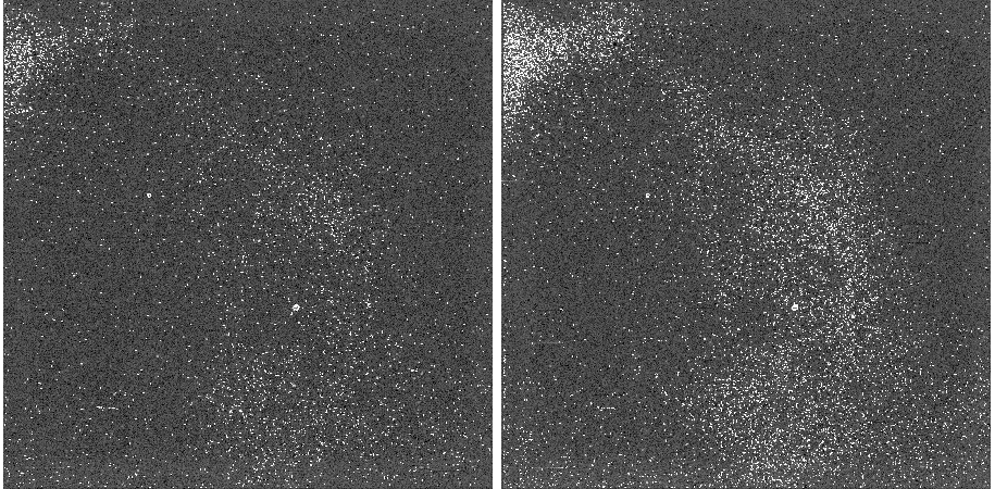
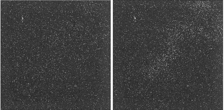
The new W3, W4 darks used in processing for the all-sky release are shown on the right in Figures 12 and 13 respectively. For comparison, we also show the darks derived from ground testing. Even though qualitatively similar, significant differences are indeed present. The flight-derived darks vastly reduced the instrumental banding structure when applied, and the impact was most noticeable in the quality of coadded image products. An overall assessment of the residual bias variations in frame products is given in section xi.1.

In closing, we mention that the darks for all bands include the constant offset term O/2^T that is added to all frames during on-board Sample-Up-the-Ramp processing (see Eq. 1 in section ii.). Therefore, this offset is automatically removed from frames after dark subtraction. The pixel values then become proportional to the photon accumulation rate.

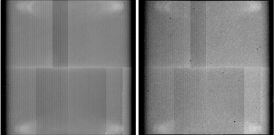Figure 12 - Dark calibration images for W3. Left: from laboratory (MIC2 testing); Right: from flight data using the method described above.

Figure 13 - Dark calibration images for W4. Left: from laboratory (MIC2 testing); Right: from flight data using the method described above.

vi. Non-linearity Calibration

The non-linearity calibration was derived from ground test data on a per-pixel basis and then validated using an on-orbit experiment. Overall, we were able to adequately linearize each array up to its saturation level as defined by the maximum signal after A/D conversion. These saturation levels were at typically ~85-90% full well across all bands. At these levels, the accuracy of the linearity calibration as determined from random statistical uncertainties and repeatability analyses of the laboratory data is ~0.31, 0.33, 0.24, and 0.62% for W1, W2, W3, and W4 respectively. Note that this ignores any possible systematic errors associated with for example how representative the laboratory measurements were of the actual flight data. Characterization of the non-linearity from flight data has proved difficult and only coarse checks with photometry at similar wavelengths from other instruments were possible. We first outline the method and summarize some results. Validation checks using color-magnitude diagnostics from source photometry are presented in section vi.1.

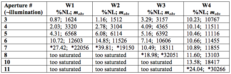
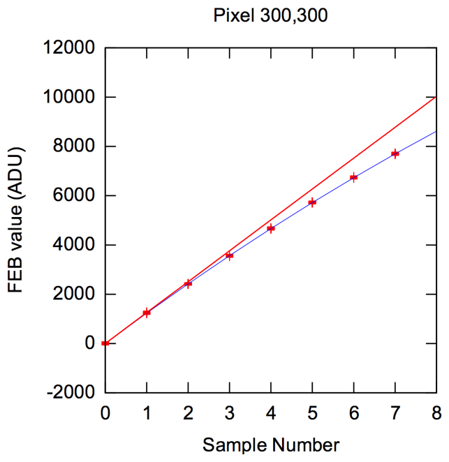
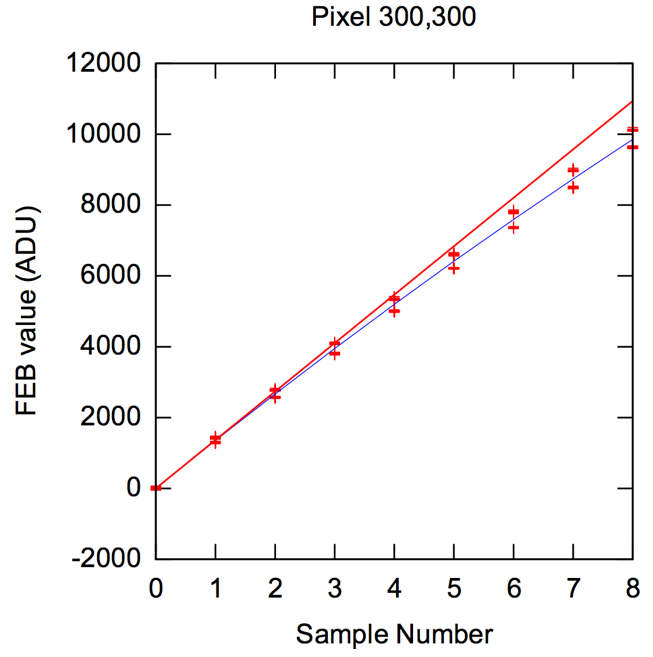
Initial analyses of Sample-Up-the-Ramp (SUR) test data for a few pixels (e.g., Figure 14) revealed that a quadratic correction model was sufficient. The method was based on fitting the SUR test data with the following model:

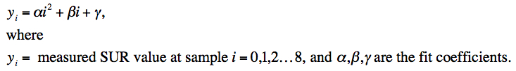(Eq. 9)

Note that the ramp intercept γ played no role in determining the ramp shape. It was simply carried along to absorb dependencies that could not be explained by α and β. The parameters α and β were estimated by fitting Eq. 9 to the ramp data y_i for each pixel using χ² minimization. The following quantity was minimized:

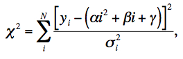(Eq. 10)

where σ_i are estimates of the uncertainties, taken as the RMS deviation in repeated exposures at each ramp sample. N was the total number of data points in the fit and included multiple ramps from repeated exposures at the same illumination. Since Eq. 9 is linear in the fit coefficients, the values of α and β that minimize χ² could be written in closed form. This is a standard textbook result and explicit solutions are not given here.

Given that Eq. 9 was fit to a specific set of laboratory data, we can generalize to any other observed ramp with underlying linear count rate β_l by scaling the "time" i at which the linear counts are equal, i.e., if βi = β_li' at times i and i', then i = β_li'/β. We can then transform Eq. 9 into a new generic expression for the counts in a ramp with linear rate β_l:

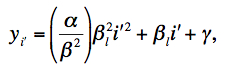(Eq. 11)

The assumption of this method should now be apparent: the quantity α/β² is assumed to be constant and independent of the incident flux. The parameter α is < 0 since the non-linear ramps generally curve downwards. This means that the fractional loss in measured counts at any ramp sample i from the linear expectation is ~ (α/β²)β_li. A higher incident flux will therefore suffer a proportionally greater loss at all ramp samples.

A linear output signal (i.e., assuming the detector was perfectly linear) can be written in terms of the true linear ramp count (β_li) and the SUR coefficients using Eq. 1 in section ii.:

(Eq. 12)

where it is assumed that a dark (and the offset term O/2^T) have been removed. On re-arranging, the true linear rate can be written in terms of the linear signal as follows:

(Eq. 13)

Substituting Eq. 13 into Eq. 11, we obtain:

(Eq. 14)

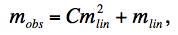
Substituting Eq. 14 into Eq. 1 from section ii. and rearranging terms, the observed signal m_obs for a pixel can be written in terms of its linearized counterpart m_lin after subtraction of the offset term O/2^T as follows:

(Eq. 15)

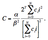
where

(Eq. 16)

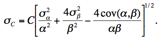
Generally we expect C ≤ 0 with C = 0 implying a perfectly linear detector. The quantity C in Eq. 16 is defined as the non-linearity coefficient and is provided (along with its uncertainty) as a FITS image for use in the ICal pipeline. The 1-σ uncertainty in C uses the error-covariance matrix of the fit coefficients and is given by:

(Eq. 17)

Eq. 15 can be inverted to solve for the linearized signal m_lin:

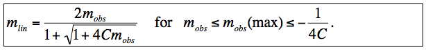(Eq. 18)

The quantity in the square root is the discriminant:

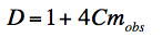and we require D ≥ 0 for a physical solution. This implies there is a maximum observed signal: m_obs = -1/(4C) above which a measurement cannot be linearized and hence could not have come from a detector with this model. It is very possible that the observed signal predicted by Eq. 15 turns-over before the maximum of the dynamic range is reached: 32752. Signals satisfying -1/(4C) < m_obs ≤ 32752 therefore cannot be linearized using this model. To avoid (or "soften" the impact of) a possible turn-over, we define the quadratic model solution in Eq. 18 to be only applicable to observed signals m_obs ≤ m_obs(max), where m_obs(max) is a new calibration parameter. For m_obs > m_obs(max), we Taylor expand Eq. 18 about m_obs = m_obs(max) to first order and linearly extrapolate to estimate the linearized signal:

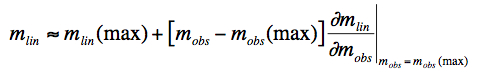(Eq. 19)

Using Equations 15 and 18, the linearized signal for observed signals m_obs > m_obs(max) can be written:

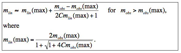(Eq. 20)

This extends the flexibility of the quadratic model and is important for characterizing the non-linearity at high signals where its effect is most extreme and there is no guarantee that it follows a simple quadratic.

The 1-σ uncertainty in the linearized pixel signal can be derived by Taylor expanding Eq. 18 about m_lin to first order, squaring, and taking expectation values to derive the variance:

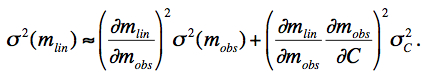(Eq. 21)

Evaluating the derivatives, the uncertainty in the linearized signal can be written:

(Eq. 22)

where σ_C was defined by Eq. 17. If the discriminant (D) in Eq. 18 is < 0, we reset D = 0 so that m_lin = 2m_obs from Eq. 18. In this limit, the uncertainty in linearized signal becomes σ(m_lin) = 2σ(m_obs).

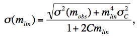
Table 4 summarizes the measured deviation from linearity using the laboratory characterization. Some notes follow below the table. W2 appears to be the most "non-linear" band at signal levels above ~10,000 DN (~70% full well). Figure 14 shows some example SUR data for a single "well behaved" pixel in each array for signal levels reaching ~55, 60, 60, 60% full well for W1, W2, W3, W4 respectively.

1. Observed signals are in DN (as output from the Digital Electronics Box [DEB] - equivalent to what one would measure in a single exposure frame). The values shown here correspond to the median signals used in laboratory testing.
2. Percentage deviation from linearity is defined as: 100*[(m_lin/m_obs) - 1]%, where m_lin = linearized DEB signal and m_obs = observed (raw) signal.
3. Asterisked numbers (*) used partial ramps with n samples where 6 ≤ n < 9 before hitting saturation after A/D conversion.

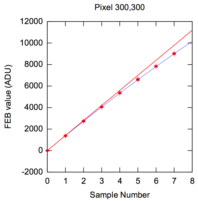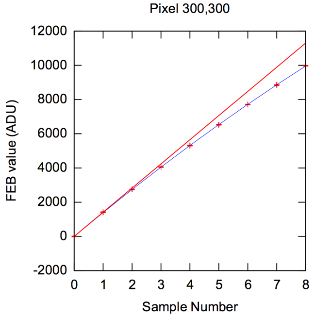Figure 14 - Example ramps for W1, W2, W3, W4 (left - right) from ground testing. Blue lines are quadratic model fits (Eq. 9); red lines are the linear components of these fits, i.e., the βi term in Eq. 9.

Figure 15 shows images of the actual non-linearity coefficient C (Eq. 16) for all bands, all on the same color scale. Note that the range of values map into the inverse of the size of the non-linearity, i.e., the darkest regions correspond to greatest non-linearity. Hence, W2 is the most non-linear overall. There is also a significant spatial variation in the magnitude of the non-linearity in each array, therefore justifying our per-pixel characterization, instead of one calibration coefficient per array. Also, there is a general tendency for pixels to be more non-linear towards the center of the W1, W2 arrays. This is reversed for W3, W4 where pixels near the edges are relatively more non-linear (by ~10%).

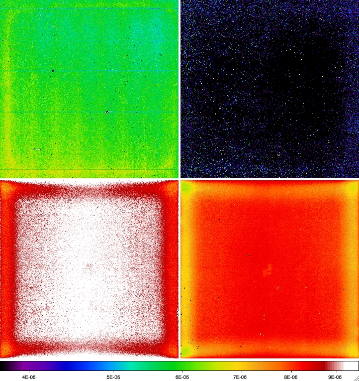Figure 15 - Images of the non-linearity calibration coefficient C (Eq. 16) for bands W1, W2 (top row), and bands W3, W4 (bottom row). Pixel values are at same stretch in all images with range represented by color-bar.

1. Validation

Figure 16 shows examples of ramps constructed using several photometric calibrators (with known brightness) for W1 and W2. The black curves are predictions from the non-linearity models presented in section iv., where the median calibration coefficient (e.g., Figure 15) over all array pixels was adopted. There is good qualitative agreement between the models and the data for these bands. A similar analysis for W3 and W4 was difficult due to the paucity of bright enough photometric standards that fell within the spatial domain of the experiment.

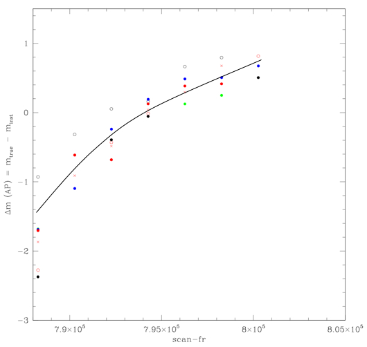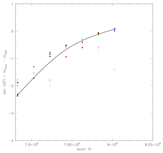Figure 16 - Left: W1 non-linearity model prediction (black curve) overlayed on trend of true - measured magnitudes of primary calibrators observed with increasing exposure time (from the on-orbit linearity experiment). Right: same plot for W2. Note: trends for W3 and W4 not shown due to insufficient numbers of calibrators.

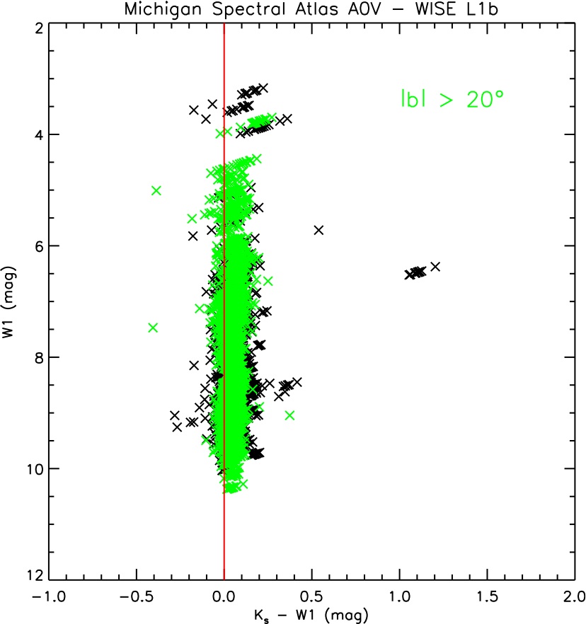
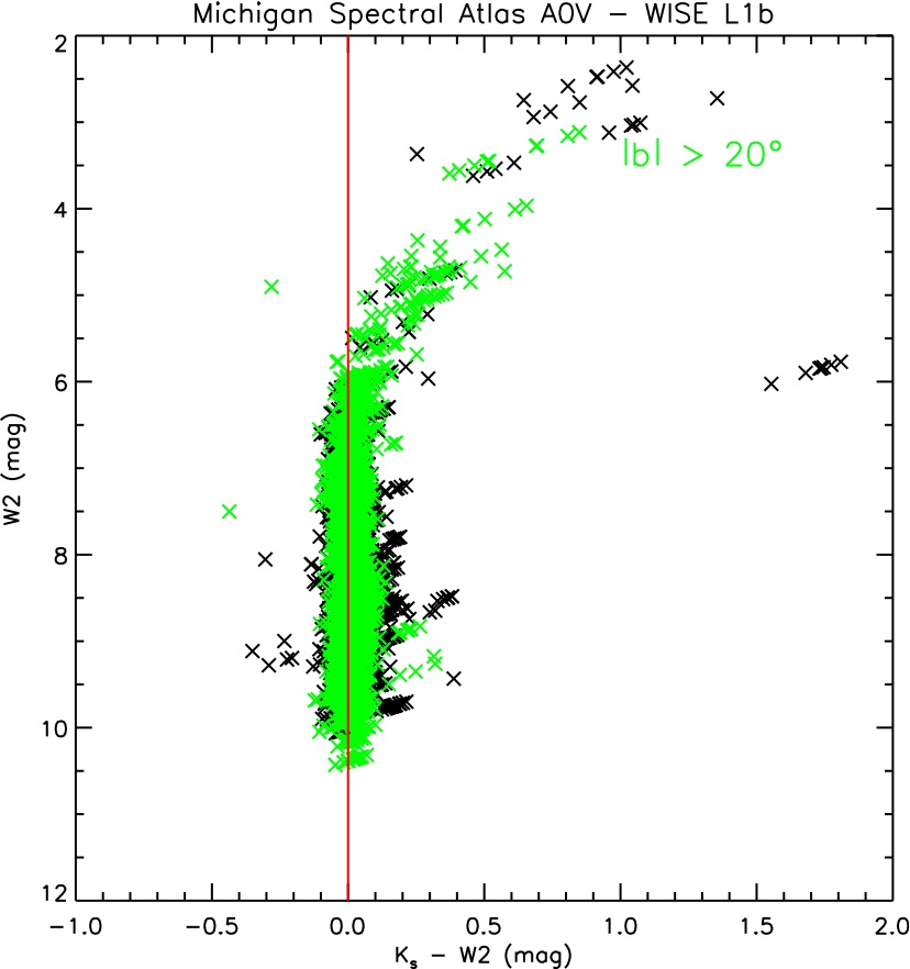
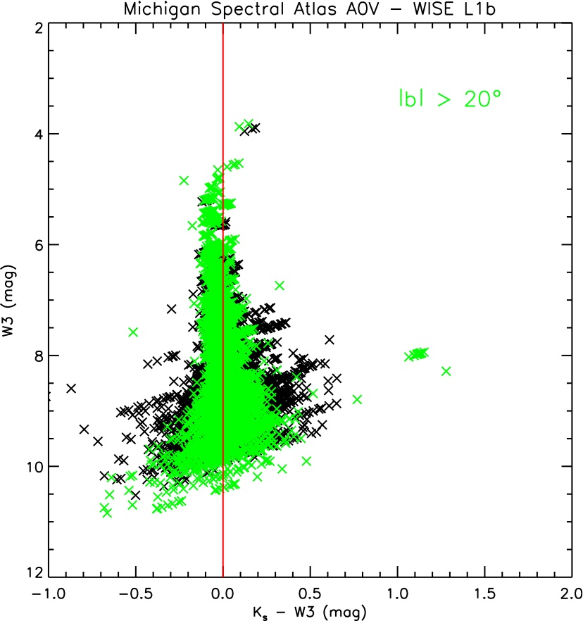
As a further check, we constructed color-magnitude diagrams (CMDs) involving 2MASS and all WISE bands for A0 dwarf stars from the Michigan Spectral Atlas (Figure 17). The WISE magnitudes are from single-exposure frame processing for the all-sky release and correspond to S/N > 3 extractions. Sources at galactic latitudes |b| > 20^o are shown as green points. Overall, even though the scatter is large, there does not appear to be a significant tilt in the color locus towards bright WISE magnitudes that may point to an over- or under-correction of flux in the WISE bands from an erroneous linearity calibration. For most bands (most notably W2), the curvature seen in K_s - WISE at bright magnitudes is not expected from the intrinsic color distribution of this population. The departure starts at approximately where saturation sets in and we have verified that it is not due to an erroneous linearity calibration. It points to an unforeseen feature of the arrays whereby the PSF becomes flux dependent at bright magnitudes. This was documented in the cautionary notes section (I.4.b).

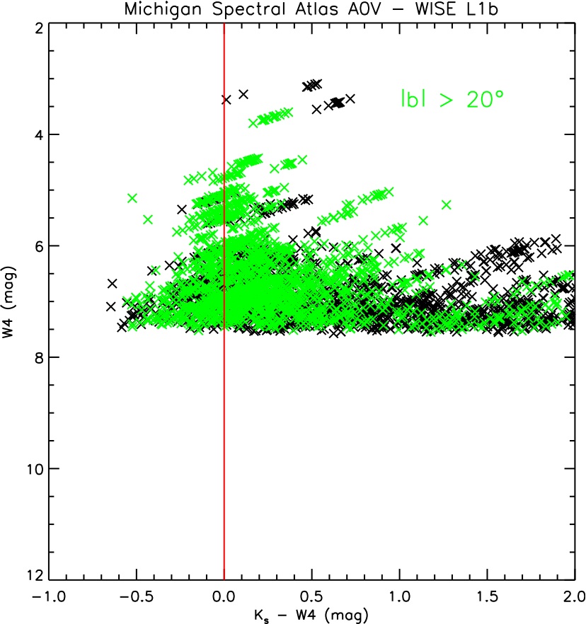Figure 17 - Color-magnitude diagrams involving the 2MASS Ks band and WISE bands: W1, W2 - top; W3, W4 - bottom, for A0 dwarfs from the Michigan Spectral Atlas. Black points are all matches and green points are for |b| > 20o. The vertical red lines at zero color are to guide the eye. The deviation in colors at bright WISE magnitudes (most extreme for W2) is discussed in section vi.1.

Lastly, Figure 18 compares photometry in W4 with Spitzer-MIPS24μm for a sample of Young Stellar Objects. Even though the scatter is large and statistics small at bright magnitudes (note: W4 enters saturation at ≈ -0.6 mag), there does not appear to be a significant deviation between these two photometric systems that may point to an erroneous linearity correction in W4.

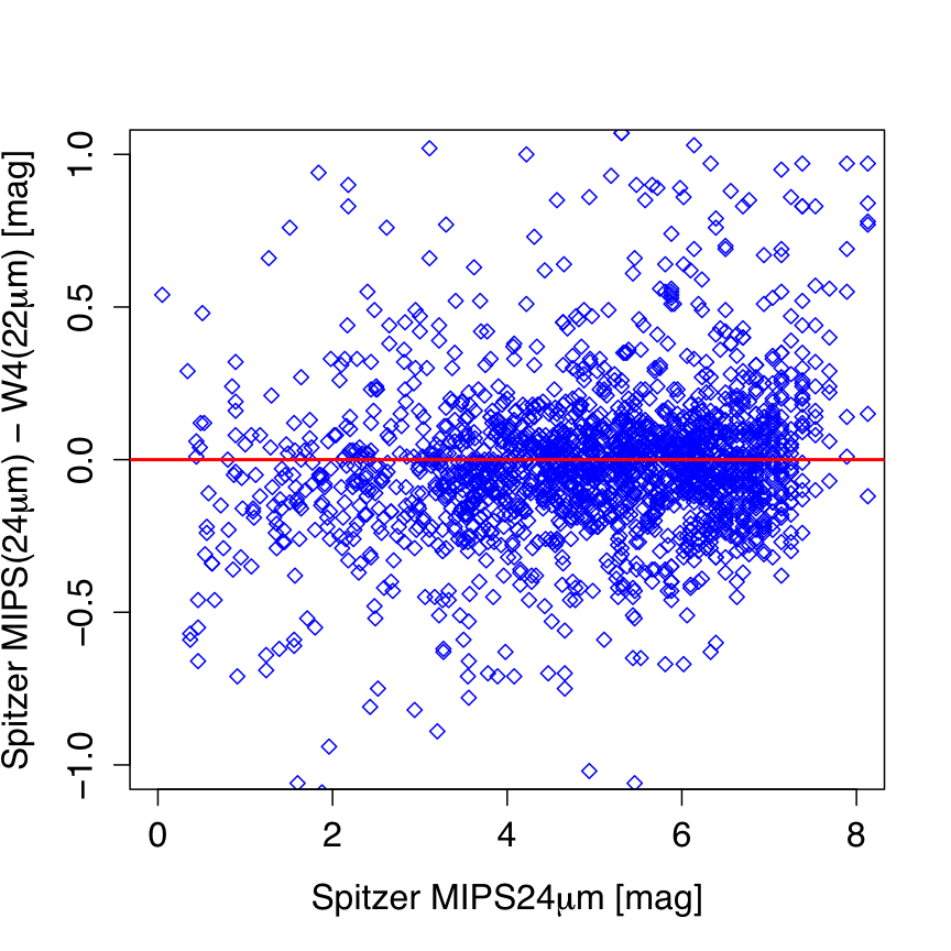Figure 18 - Magnitude difference using Spitzer MIPS24μm band and W4 (22μm) versus MIPS24μm magnitude for a sample of Young Stellar Objects. Red line is to guide the eye.

vii. Relative Responsivity (Flat-field) Calibration

Flat-field calibration images for all bands were created directly from the on-orbit survey data. No separate dedicated data were acquired on orbit for the flat-field calibration. Below we describe the methods used. The relative flat-fielding accuracy achieved in each band is summarized in section vii.2.

1. Methodologies

In order to check the temporal stability of the flat-field, one flat-field image was created from each month of data in the cryogenic mission. It was determined that all observed variations between these flat-field images was due to the changing illumination pattern of the Galactic background, and not a time-varying pixel response. Hence, a single static master flat-field was created for each WISE band utilizing all of the data from the cryogenic mission.

Two different methods were employed to create the flat-field images for W1 & W2, and W3 & W4, respectively. For W1 & W2, a frame-stacking method was implemented as follows. A dark image was subtracted from each of the input frames, then each frame was pre-normalized by its respective median pixel value. An outlier-trimmed average was computed for each pixel stack and the resulting image was normalized by its median value to create the normalized flat-field image. In addition, a corresponding uncertainty image was created by dividing the trimmed stack standard-deviation image by the square root of the stack-depth at each pixel. Approximately 50,000 input frames were used in the creation of the flat-field images, evenly distributed in time across the cryogenic mission but excluding frames at low Galactic latitudes and those impacted by the moon. The final flat-field and uncertainty images for W1 and W2 are displayed in Figures 19 and 20, respectively.

Figure 19a - W1 Flat-field image	Figure 19b - W1 Flat-field uncertainty image
Figure 20a - W2 Flat-field image	Figure 20b - W2 Flat-field uncertainty image

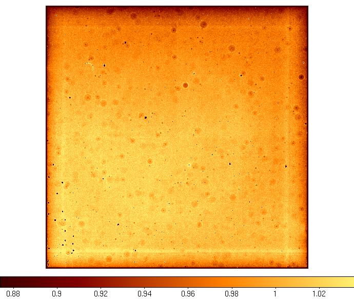
For W3 & W4, flat-field images were created by measuring the change in intensity in a pixel in response to the variation in overall intensity on a frame as the uniform illumination on the array from the zodiacal background varied. The relative responsivity for a pixel is given by the slope of a linear fit to the pixel versus overall frame intensity. This "slope" method helps mitigate incomplete knowledge of the static absolute dark/bias level. For W3 & W4, a more careful selection of input frames was performed than for W1 & W2. Latent images of celestial sources that persist on both short and long time scales were found to pose a particular challenge to creating "clean" flat-field images. W3 & W4 were annealed about every 12 hours to periodically remove these accumulating latents. However, since the responsivity itself changed as a function of time since an anneal, we compromised and selected frames relatively close to anneals in order to have as few latents as possible, but not too close to be affected by the responsivity-altering behavior of the anneal itself. Like W1 & W2, frames at low Galactic latitudes and those affected by the moon were excluded from the input list. Due to the tighter selection criteria, only about 17,000 frames were used for W3 & W4. The final flat-field and uncertainty images for W3 & W4 are shown in Figures 21 and 22, respectively.

Figure 21a - W3 Flat-field image	Figure 21b - W3 Flat-field uncertainty image
Figure 22a - W4 Flat-field image	Figure 22b - W4 Flat-field uncertainty image

2. Flat-fielding Accuracy

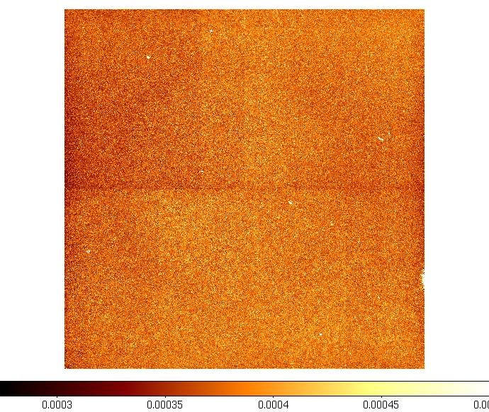
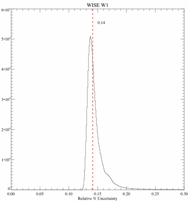
An estimate of the flat-field accuracy is provided by the relative percent uncertainty derived from the uncertainty images. This is defined as the median of 100 * [σ(f) / f] over all the pixels where σ(f) is the 1-sigma uncertainty in the responsivity f for a pixel. The median relative percent uncertainties for all WISE bands are listed in Table 5. Histograms of the relative uncertainty per pixel are shown in Figures 23 - 26.

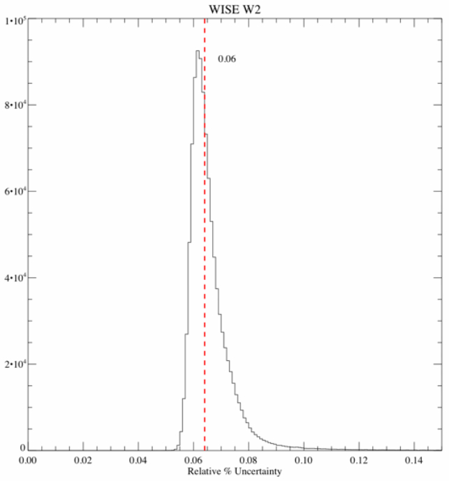Figure 23 - Histogram of relative % flat-field uncertainties for W1	Figure 24 - Histogram of relative % flat-field uncertainties for W2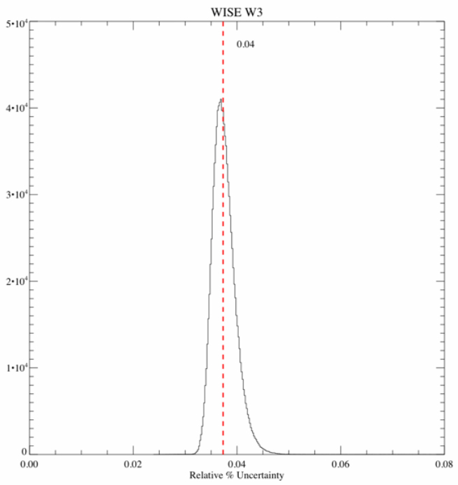
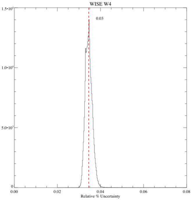Figure 25 - Histogram of relative % flat-field uncertainties for W3	Figure 26 - Histogram of relative % flat-field uncertainties for W4

viii. Dynamic Calibration

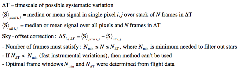
The purpose of dynamic calibration (dynacal) is to capture instrumental transients in the WISE detectors and then correct them in the frames from which the calibrations were made. Dynacal is a seperate pipeline that executes some of the pre-calibration steps of the ICal pipeline (Figure 1) to provide the input frames for creating the dynamic calibrations in a module called dynasky. The inputs were mainly dark-subtracted, linearized, and flat-fielded using static calibrations. Dynacal generates three products per frame: (i) a "sky-offset" image (all bands) from a running median of N consecutive time-ordered frames along a scan, forced to have zero global median; (ii) a low-frequency delta flat-field image (bands W3 & and W4 only) from the same running median to capture spatially extended elevations in responsivity brought about by long-term latents; (iii) a transient bad-pixel mask (all bands) that stores new bad pixel information. "Bad" here refers to pixels whose values persist in a high or low state for several consecutive frames centered on the frame of interest. We discuss each in turn below.

1. Sky-offset Correction

The goal of this correction is to capture short-term variations in the bias and dark structure that could not be corrected by the static long-term dark calibrations. These variations were mitigated by first computing a stack-median of ~30 median-subtracted frames in a single frame-step moving window along the WISE orbit, after filtering bad and unusable frames, e.g., due to very high source density, complex backgrounds, and/or severe moon glow. The pixel-median was then subtracted from this "sky" image to create the "sky-offset" image. This image was then subtracted from each respective (window-centered) frame in a subsequent run of the ICal pipeline. We needed to stack at least ~30 frames per window to reliably filter out sources in any band. This number therefore became the shortest characteristic time scale: 30 x 11 sec/frame ~ 5.5 min (or ~ 5.4% of a WISE orbit) on which to capture possible instrumental variations. A one-dimensional schematic of the sky-offset cencept is given in Figure 27. As a detail, if a sky-offset cannot be made due to an insufficient number of frames after filtering, the "best" closest-in-time product (either forwards or backwards in time) within a maximum time interval is adopted. This scheme also applies to creation of the delta-flat discussed in section viii.2.

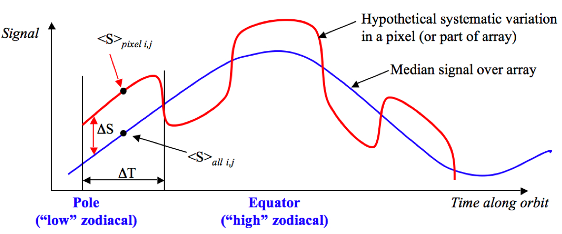Figure 27 - One-dimensional schematic illustrating the concept of the sky-offset calibration. Symbols are defined below.

Labels and symbols in Figure 27:

2. Band 3 and 4 Delta-flat Correction

Using the same infrastructure and windowing scheme as for the sky-offset calibration (section viii.1), we also generate low spatial-frequency delta-flats from the pre-flattened input frames (made upstream using a static flat). These are "low spatial-frequency" images in that the goal is to capture spatially extended elevations in responsivity (of up to 10%) due to long-term latent artifacts affecting the W3 and W4 arrays and persisting until the next anneal on a 12hr cycle. The input frames are first normalized by their median, filtered for bad cases (as above), then median-stacked in a 30-frame, single frame-step moving window. The product is then renormalized by its median to yield essentially a (delta-)flat storing all the relative pixel-to-pixel responsivities. This is then converted to a low-frequency delta-flat by retaining only pixel values with a relatively high (>2%) response and then resetting all lower response pixels with the value 1. The pixels with a high relative response are usually in clusters (or blotches) falling on the long-term latents sought for (e.g., Figure 28). To ensure that the latent regions are captured completely (i.e., down to their low edges), a filter is applied to slightly expand the size of retained/thresholded regions in the delta-flat.

As mentioned in the cautionary notes section (I.4.d), there are three anomalies associated with the application of dynamic calibrations. All are very subtle and rare, but if present, will impact photometry off the single exposure frames.

1. Dark residuals are sometimes seen in W3 and/or W4 frames at the array positions of ultra-bright stars that occur in future frames. This backwards-in-time crosstalk is due to over-correction by the dynamic delta-flat in frames prior to the latent-inducing bright-stars since they were included in the dynamic calibration window.


2. There are instances when dynamic calibrations (both sky-offsets and delta-flats) could not be made from frames crossing dense regions of the galactic plane. This was intentional since a high source density would have lead to bad calibrations and hence a large number badly calibrated frames. Therefore, expect to see floating long-term latents in W3 and W4 frames in some regions of the galactic plane.


3. On some occasions, the Si:As detectors (serving W3 and W4) exhibited a transient elevation of responsivity around their edges relative to their center. These manifested as artifacts around the edges of calibrated frame products following application of a dynamic delta-flat that is only intended to mitigate elevations in responsivity due to long-term latents. These residuals are a limitation of the thresholding used to create the delta-flats. The high-edge responsivities were not preserved in the calibration products to enable their removal. The residuals are multiplicative and when present, are generally at the <~4.5 and <~3% level in W3 and W4 frames respectively.

Overall, the dynamic calibrations improved the photometric accuracy in all bands by a few to several percent. For W3 & W4 the benefits from the delta-flat in particular were huge. This significantly improved both the photometric accuracy of real sources superimposed on long-lived latent artifacts (with elevated responsivity), and the reliability of source detections for the Source Catalog. The nature of these long-lived latents is further described in section IV.4.g.iv.2. These latents persisted long enough (until the next anneal) to be captured and removed on a per-frame basis. Some of them (mostly the strongest) were also caught by our transient bad-pixel detector (section viii.3), and tagged in the frame masks. Figure 28 shows a blink animation of a frame processed with and without the dynamic calibrations (sky-offset and a delta-flat). The long-term latents appear as fuzzy entended blotches in the uncorrected frame.

Figure 28 - Click for a blink-animation of a W3 frame processed with no dynamic calibrations (hence containing long-term latents) and the same frame corrected using dynamic calibrations. Green regions in the corrected frame are bad pixels.

3. Transient Bad-pixel Masking

Transient bad-pixel masking attempts to tag pixels which become hot or unresponsive for a period of time, or remain so for the duration of the mission. The static bad-pixel masks (section iii.1.) only record those pixels which are known to be "bad" a apriori from analysis of all the static calibrations (Table 1). Our transient detection method still has its limitations, e.g., it is only sensitive to high and low pixel excursions from normality, but only if they stay this way for a consecutive run of ≥ 11 frames (for the all-sky release). This includes the occasionally strong long-lived latent (see also viii.2). Pixels which become transiently noisy and fluctuate wildly on shorter timescales will escape detection.

The method uses the fact that bad pixels are always at the same x, y location in a set of frames, whereas astronomical sources move around as the frames are dithered or systematically offset from each other on the sky. Therefore, if a pixel is detected as an outlier with respect to its neighbors in a given frame, and it persists in this state (as an outlier) for the next consecutive N frames, it can be identified and tagged. The spatial outlier-detection is performed by first subtracting a smooth varying background from a frame, robustly-estimated over a 8 x 8 grid (all bands), and then applying robust statistics to the pixel distribution in each grid square to find the outliers. This is repeated for all N frames in a time-ordered sequence, i.e., in a moving window with a step-size of one frame. If the same outliers occur at the same x, y position for N ≥ 11 frames in succession, the pixels are tagged with bit #21 in the mask corresponding to the center-window frame. The window then advances ahead one frame and the process is repeated until all frame masks are updated with possible transients.

ix. Spatial-outlier (Glitch) Masking

This step is "orthogonal" to (and complements) the temporal (frame-stack) outlier detection method described in section IV.4.f.v. The spatial-outlier detection method in ICal operates on a single frame basis and is designed to catch and tag (in the accompanying frame mask) abnormally high/low pixel spikes and small "hard"-edged pixel clusters. This step is performed after all instrumental calibrations have been applied, but before selected bad pixels are replaced with NaNs in the final frame.

There are two input parameters controlling the detection of hard-edged pixels: (i) a threshold, trat, for the ratio:
R = "regularized pixel value / local median filtered value at pixel location",
and (ii) a linear kernel size n (where n ≥ 3 pixels) specifying the size of the n x n median filter. If R exceeds trat, the pixel is declared an outlier and tagged as bit #28 in the frame mask.

The regularized pixel value in R is defined as abs(input pixel value - background) + 1, where abs is a function returning the absolute value of the argument. The background is estimated by computing medians within squares over a 10 x 10 grid on the frame. This block-median image is subtracted from the input frame and a constant of 1 is added. This constant is to avoid inadvertent division by zero when the background-subtracted frame is divided by the local median filtered image. The local median filtered image is computed using a 5 x 5 kernel. This operation replaces each pixel by a median of its neighbors and itself. The threshold for R and median-filter kernel size were tuned such that pixels with soft-edges were avoided, i.e., with neighbors whose signal declined no faster than the wings of the critically sampled PSF for the respective band.

x. Band 1 and 2 Channel-noise and Bias Corrections

These corrections attempt to fix four main problems with the W1 and W2 detector arrays. These are labeled in Figure 29a as follows:

1. Bulk channel fluctuations (or "channel-droop"): sometimes the entire channel is brighter or darker than the rest in an image, which appears as a dark or bright band in the images. The amplitude in either direction can be as much as 6 DN. The reference pixels on the ends of the channels typically reflect this offset.


2. Inter-(along)-channel noise: in both W1 and W2, amplifier channels often have alternating pixel row/columns of brighter or darker signals than normal. The amplitude of the variations appears to be constant in a given channel of a frame. The full amplitude can be as much as 8 DN, with W1 typically having higher amplitudes than W2. Furthermore, the first and last two rows/columns of a channel can have a spike either significantly brighter or darker than the rest of the channel. This can appear as bright or dark lines between each channel in the image.


3. High frequency cross-channel noise: this can be seen as faint lines extending across all channels in both W1 and W2. Fourier analysis reveals that there is an underlying sinusoidal pattern with sharp peaks superimposed. This noise pattern appears very stable across all frames. The wavelength in pixel space is 44.44 pixels and appears to move in the same direction at 0.6849 pixels/sec. Thus, the wave passes through the same phase value every 64.89 seconds, or some integer harmonic. The full amplitude of the sine wave is approximately 0.8 DN and the full amplitude of the peaks is about 3.5 DN.


4. Low frequency cross-channel noise: this is only present in W2 and can be seen as broad lines extending across all channels. It is not always present and is unstable. Unlike the high-frequency noise, this feature changes wavelength between survey scans, ranging from 125 to 150 pixels. The wave appears to move in the opposite direction of the high frequency noise, though velocities close to integer harmonics of the wavelength can make the wave appear to move in either direction. The wave velocity is usually stable for most of a survey scan, and often appears to increase near the end of a scan. When stable, the velocity is approximately 2.6 pixels/sec, and thus has a cycle time of ~48 to 58 seconds. The average amplitude of the wave is about 2.3 DN, but sometimes the amplitude is higher in certain channels. The frequency appears to always be the same in a given scan.

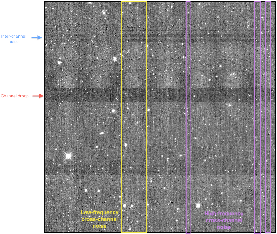Figure 29a - A single exposure for W2 with the four main issues labeled. All features except for "low frequency cross-channel" noise are also seen in W1. Click to enlarge the labels.

The cross- and along-channel high frequency patterns are corrected by first collapsing each channel in its row and column directions separately using a median. These 1D-collapsed sequences are smoothed using a median filter to obtain the underlying signal baselines and then subtracted from the original 1D sequences to create two correction vectors per channel (for the row and column directions). These correction vectors are then spatially stretched across the rows or columns of a channel and applied (subtracted) from all its pixels to smooth out the noise. Corrections are not applied to pixels containing a "high" signal that may be associated with a real source. The high signals (relative to the background) are detected by also computing 1D-collapsed row/column sequences using an average instead. The high source signals will bias the average values relative to the median collapsed values, therefore enabling one to tag the high signals for omission from the corrections. The low-frequency cross-channel noise (for W2 only) is corrected using a similar procedure but with a longer-length median filter applied to the 1D-collapsed sequences to capture the sinusoidal pattern with respect to the underlying background.

The bulk channel fluctuations are corrected using relative corrections computed from the reference pixel signals at both ends of a channel. The median reference pixel value for a channel is subtracted from the median of all the channel-reference pixels to construct a delta correction. If this delta exceeds some threshold, we then check if a fluctuation of similar magnitude and sign also occurred in the median signal of the active part of a channel relative to its adjacent channel(s). If this active-pixel median delta exceeds another threshold (different from the reference pixel threshold), the correction derived from the channel-reference pixels is applied to the respective active pixels. This is performed for all channels.

Figure 29b compares a collection of W2 frames with and without channel-noise corrections applied. The improvement is most apparent in the intra-channel, high frequency cross-hatching effect. The bulk channel-bias fluctuations are corrected to an accuracy determined by the noise in the (small number) of reference pixels above/below each channel (whose values are quantized to +/- 1 DN), and the degree to which they correlate with the active pixels. This explains the residual bulk-channel variations sometimes seen W1 and W2 frames. Overall, we find that the local RMS noise in both bands is reduced by ~4-5% compared to products where no channel-noise/bias corrections were applied (e.g., products from the preliminary data release).

Figure 29b - top row: collection of W2 frames from the preliminary data release (initially processed without correcting for channel-noise); middle row: the same frames processed for the all-sky data release with the same image stretch; bottom row: differences between the images in the previous two rows, where the color bar spans -4 to 4 DN.

xi. Instrumental Calibration Performance

In this section, we present some analysis to assess the accuracy of the calibrations in removing instrumental residuals from the single-exposure image products in the all-sky release. We used two methods: (i) examined the magnitude and variation of spatial "bias" (or offset) residuals by collapsing background-normalized frames along their column or row directions and stacking the results from thousands of frames, and (ii) explored the spatial variation in "multiplicative" residual structure, i.e., the accuracy of the relative responsivity (flat-field) corrections.

In summary, residuals in the bias structure are at a level of <~ 0.20%, <~ 0.14%, <~ 0.007%, and <~ 0.016% for W1, W2, W3, and W4 respectively. These estimates use the maximum residual values from the analysis in section xi.1 divided by the lowest background signals observed (conservatively speaking), which typically occur at the ecliptic poles. The residual biases in W1 and W2 are dominated by high-spatial frequency structure within the amplifier channels (section x.). Residuals in the relative pixel responsivity (section xi.2) are at a level of <~ 0.7%, <~ 0.2%, <~ 0.23%, and <~ 0.25% for W1, W2, W3, and W4 respectively. These estimates are 95^th percentile upper limits in the value |r - 1| where r is the relative responsivity as shown in Figures 34 and 35.

1. Analysis of Spatial-Bias Residuals

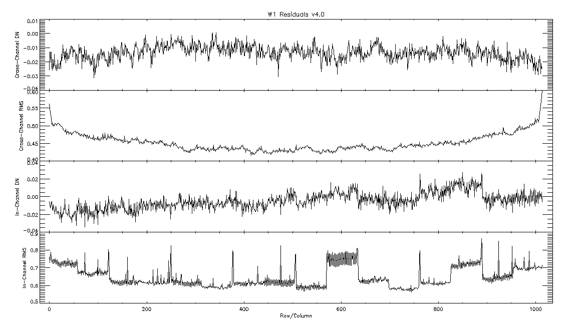
To quantify the effectiveness of the instrumental calibrations in removing systematic spatial structure over a frame, residual plots were generated using a "supermedian" stacking method. These supermedians are plots of the global median of the median-collapsed pixel values along the row or column direction over a large number of calibrated frames. They are useful to visualize residual spatial variations that occur along the row or column-pixel direction in general. For W1 and W2, the median of the entire frame is first subtracted from each row or column median so the values are robust against sky-background variations. For W3 and W4, the same is done for each individual quadrant instead of the entire array. The RMS of the supermedian value is also computed. This gives a measure of the sensitivity and noise of each row or column. For this analysis, data from ~20,000 frames were combined for each band. Furthermore, frames with an array median ≥ 2000 DN were excluded from the analysis to ensure that cases with high nebulosity, moon-glow artifacts, galactic plane crossings, and frames acquired shortly after an anneal (for W3 and W4) did not skew the results.

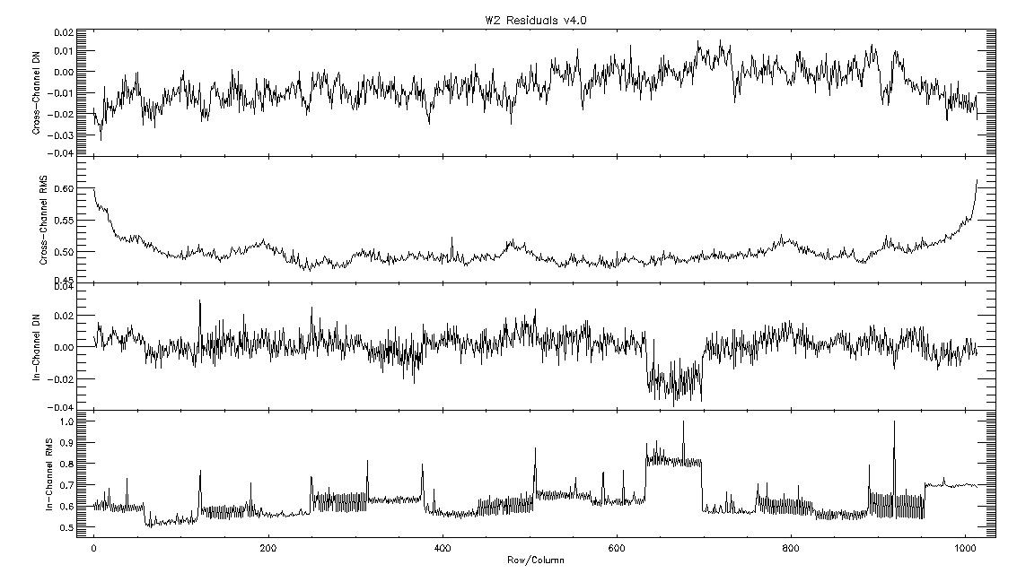
Figure 30 shows the supermedian analysis for W1. The top panel shows the residual signal in DN for each row of the array (the cross-amplifier channel direction). There is little variation. The second panel down in Figure 30 shows the RMS of the medians of each row. The array is slightly more stable towards the center with the RMS ≈ 1.4x higher at the edges. The third panel down shows the in-channel (column) residuals. The bottom panel shows the RMS of the in-channel residuals. Amplifier channels 1, 10, and 14 are particularly noisy, and the inter-channel noise (section x.) is quite evident in both the RMS and residual plots. The same analysis was done for W2 as shown in Figure 31.. For W2, channel 11 appears to be the noisiest.

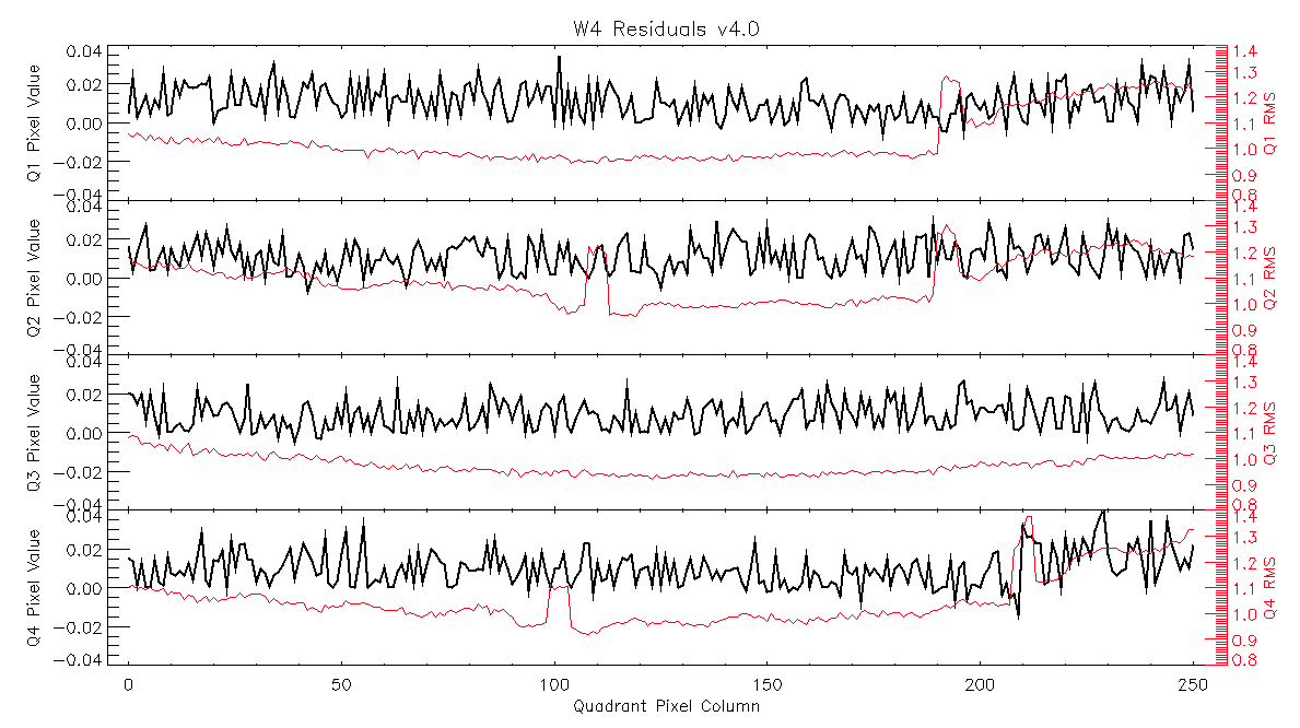
The analysis for W3 is shown in Figure 32. Here, the medians were computed for each quadrant, and only for columns, as the majority of the droop-related corrections are applied to the columns, not rows. The four panels show the results for each of the four quadrants. The black line and left axis are the residuals in DN, while the red line and axis are the corresponding RMS. Interestingly, the RMS dips in the middle of each quadrant, thus the array seems to be more stable (hence more sensitive) at the center of each quadrant than at the center of the full array. The residuals are less than 0.05 DN for all quadrants. The abrupt jumps in the RMS and residuals are due to the banding pattern seen in the W3 dark. Figure 33 presents the same analysis for W4 where results are similar to W3.

Figure 30 - W1 supermedian analysis. From top to bottom: cross-channel residuals, cross-channel RMS, inter-channel residuals, and inter-channel RMS by row/column number.	Figure 31 - W2 supermedian analysis. Panels are the same as in Figure 30.
Figure 32 - W3 supermedian analysis. The four panels correspond to quadrants 1-4 from top to bottom. The black curves and left axes are the residuals for each column, and the red curves and axes are the corresponding RMS.	Figure 33 - W4 supermedian analysis. Panels are the same as Figure 32.

2. Analysis of Spatial-Responsivity Residuals

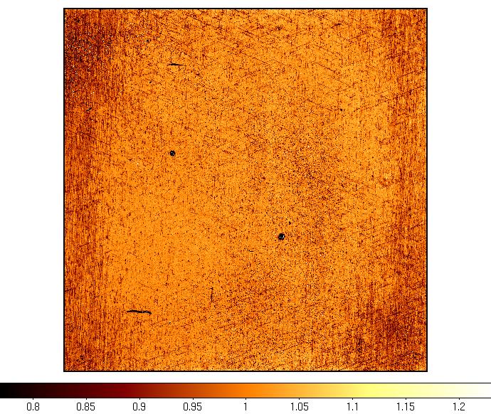
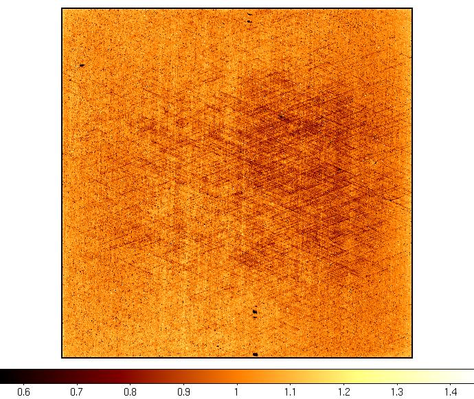
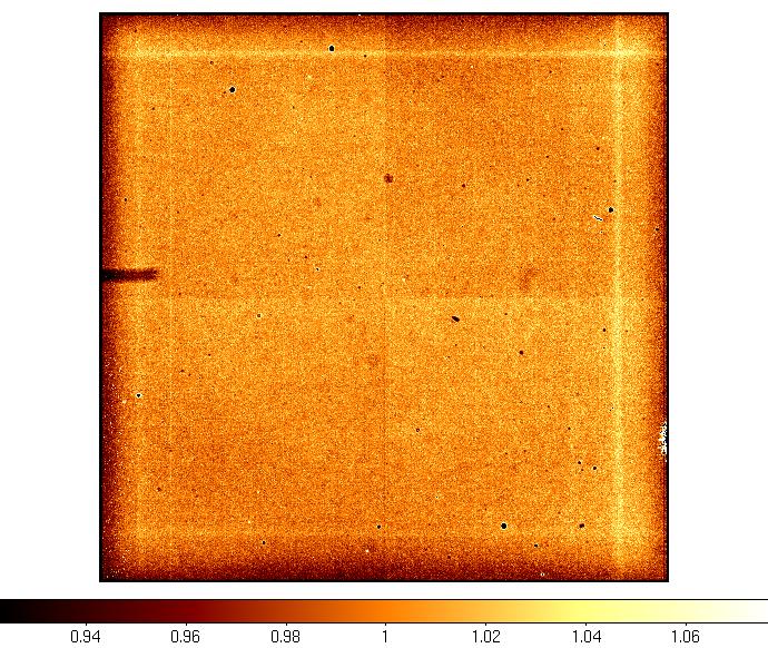
Residual flat-field images were made by median stacking several thousand instrumentally calibrated frames in each band. The images were normalized by their global median to yield relative pixel responsivities. If our dynamic and static flat-field calibrations were perfect (i.e., captured all spatial and temporal variations), the residual flat-field images would be equal to unity. However, slight variations are seen that are well within the requirements for photometric repeatability. Figure 34 shows the residual responsivity maps for bands W1 and W2 where variations are well within 0.8%. Figure 35 shows the same for bands W3 and W4 where variations are within 0.25%.

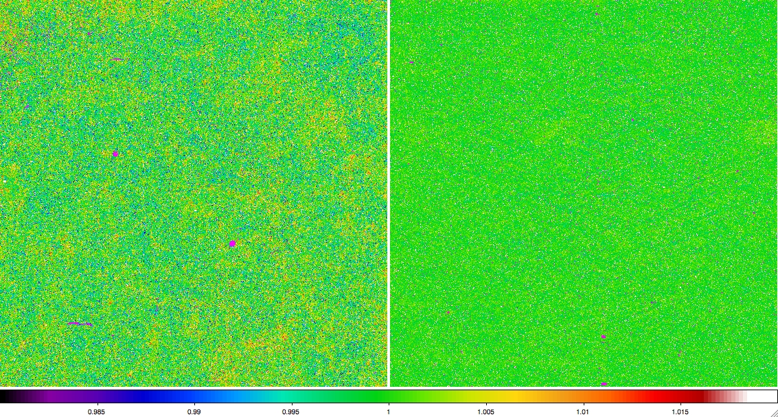Figure 34 - Residual responsivity map for W1 (left) and W2 (right). Color bar shows the range of values (~1.5% peak-to-peak).

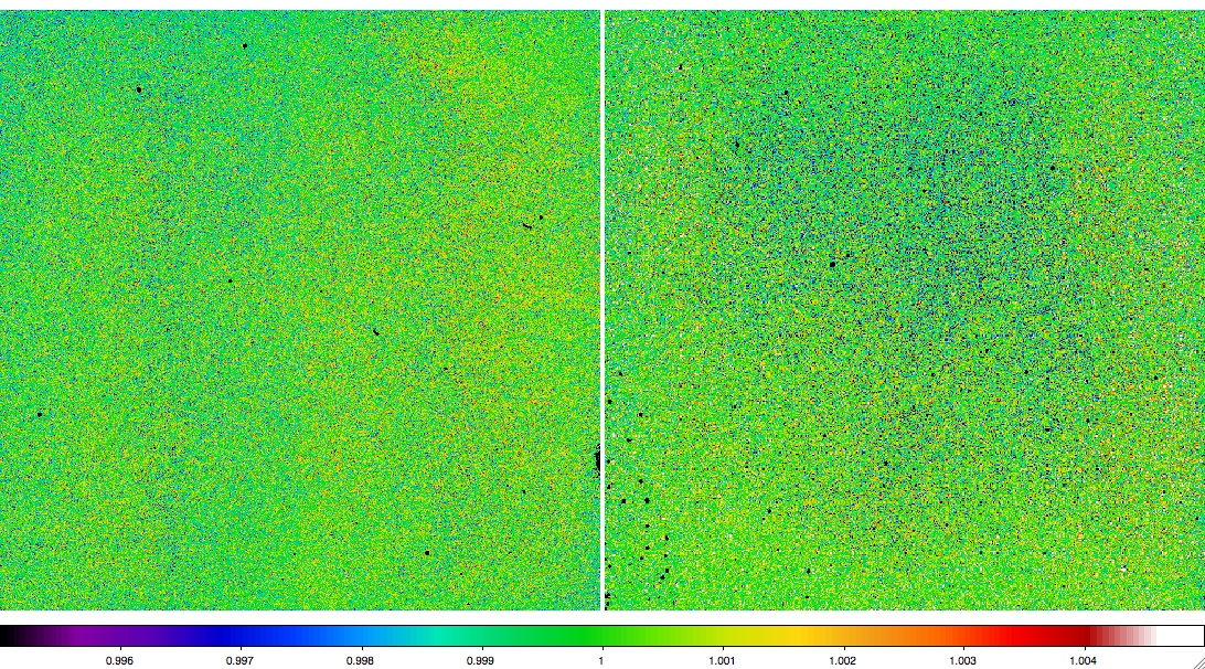Figure 35 - Residual responsivity map for W3 (left) and W4 (right). Color bar shows the range of values (~0.4% peak-to-peak).

Last update: 2012 March 15