
| Use of Interpolation (Smoothing) Kernels in Coverage Simulations | |
Interpolation kernels will be used in the co-addition process for optimally generating WISE Atlas images. The best interpolation kernel for this process is represented by the Point Response Function (PRF). The PRF gives the distribution in the fraction of flux over the sky collected by a pixel. The PRF is usually unit normalized, and can be computed by convolving an instrument's Point Spread Function (PSF) with the shape and size of the measurement pixel (a square or box function in 2D). In the limit of dense over-sampling of the PSF (much above the Nyquist limit), the PRF becomes in principle the PSF. In the limit of extreme under-sampling of the PSF (much below critical), the PRF takes on the shape of the boxy pixel itself, which is the most "compact" PRF possible.
When used in the co-addition process, interpolation kernels have the effect of smearing (or smoothing) information collected by "good" pixels over the sky. Since source detection will primarily occur off the WISE Atlas images, the impact of kernel smoothing on the effective depth-of-converage in the presence of bad pixels must be deduced. This will enable a more reliable estimate of the sensitivity.
Below we summarize the assumptions and analytical approximations used to define interpolation kernels for each WISE band. These approximate kernels are only used for simulating the achievable depth-of-coverage. They will not be accurate enough for co-adding real image data acquired with WISE. The coverage simulations that use these kernels are presented on the following pages:
Coverage simulations for fpa 141.
Coverage simulations for fpa 143.
Coverage simulations for fpa 143 at reduced bias.
Coverage simulations for all flight and spare arrays.
At the time of writing, PRFs derived from optical + detector characterization of the WISE flight system were not available. Instead, we used a simple 2-parameter model for the PRF in a given band. A model PRF profile is determined by convolving a 2D symmetric Gaussian for the PSF with a square pixel response:
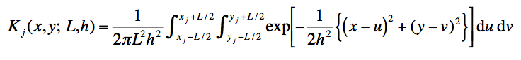 |
(Eq. 1) |
where (xj, yj) is the center of the jth pixel with linear scale L = 2.75 arcsec, and h is the second moment σ of the underlying PSF. Given that we assumed a Gaussian for the PSF, the FWHM of this PSF is ~ 2.354h. On integrating, the PRF kernel becomes:
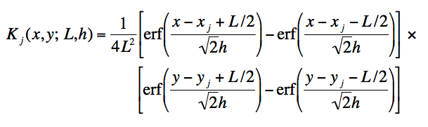 |
(Eq. 2) |
Eq. 2 represents the contribution of the flux falling at some arbitrary point (x, y) to the measurement in a pixel centered at (xj, yj). The kernel is unit-normalized. This construction is similar to that adopted in 2MASS processing (2MASS Atlas Image Generation).
Given the nominal pixel size L, the only dependent parameter is h (~FWHM(PSF)/2.354). This parameter is estimated, and hence the ultimate model kernel constrained by solving for h until Eq. 2 predicts the expected number of "noise pixels" Np for the WISE arrays.
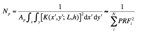
The number of noise pixels, Np, is the number of pixels in an aperture whose total uncertainty (summed in quadrature and assumed independent) matches the uncertainty in a point source flux F derived from a PRF-weighted fit in that aperture. Put another way, it is the number of pixels such that the variances are related by σ2F = Npσ2pix . Np gives an alternative measure of the effective size of the PRF, and is the metric of choice for optical/detector performance. In general,
 |
(Eq. 3) |
where Ap is the active area of a pixel (Ap~1 for a PRF kernel K in units of pixel-1). For a top-hat PRF normalized to unity such that PRFi = constant = 1/N for all N pixels in an aperture, Np = N.
We use the predicted values of Np
from Mark Larson's June 2007 CDR presentation together with
Eqs 2 and 3 to estimate effective FWHM values of the underlying PSF
and PRF kernels in each WISE band. Results are shown in Table 1.
Figure 1 shows the number of "noise pixels" predicted using the
PRF in Eq. 2 as a function of the FWHM of an underlying Gaussian PSF.
| Band | Np1 (# noise pixels) |
PSF FWHM2 (arcsec) |
PSF FWHM3 diff. limit (arcsec) |
PRF FWHM4 (arcsec) |
|---|---|---|---|---|
| 1 | 11.4 (14.7) | 5.8 (6.7) | 1.71 | 6.1 (6.9) |
| 2 | 14.6 (18.3) | 6.7 (7.6) | 2.44 | 6.9 (7.9) |
| 3 | 39.0 (45.1) | 11.3 (12.1) | 6.24 | 11.5 (12.3) |
| 4 | 27.3 (28.9) | 18.6 (19.2) | 11.95 | 18.9 (19.6) |
| Figure 1 - The number of "noise pixels" as a function of the FWHM of an underlying Gaussian PSF derived using Eqns 2 and 3. Assumes 2.75 arcsec pixels. |
Once a model for the PRF kernel for a specific band is determined (by constraining Eq. 2 from the predicted "noise pixels"), we pixelate it so it can be applied to (or convolved with) a bad-pixel mask for input into the coverage simulator. We pixelate the kernels by sampling and integrating over a 9x9 pixel grid, and then renormalizing to 1. The following sections show the model PRF kernels used in the coverage simulations.
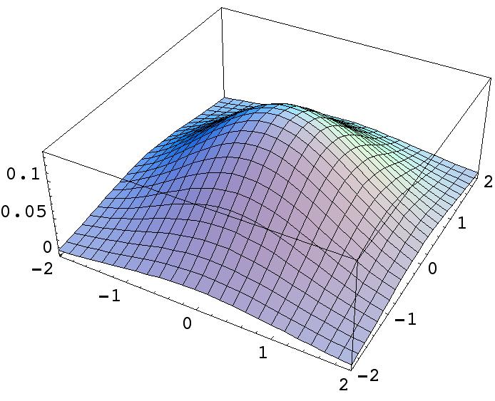
The pixelated model PRF kernel (normalized to unity) for band-1 using the above construction is as follows. This is based on integrating the kernel shown in Figure 2 over a 9x9 detector pixel grid centered at (0, 0).
0.0763923  0.123607  0.0763923
0.1236070  0.200003  0.1236070
0.0763923  0.123607  0.0763923
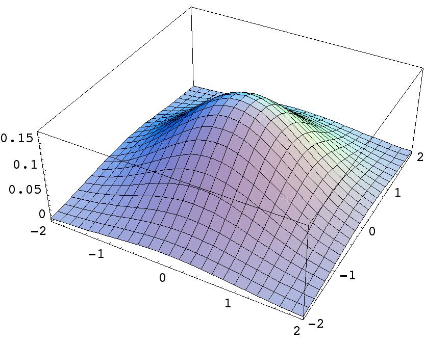 |
| Figure 2 - Model PRF kernel (Eq. 2) for WISE band-1. The area (or volume) under the function is unity. The x and y axes are in detector pixel units. The mesh shows the contribution of the flux at some point (x, y) as measured by a pixel centered at (0,0) and covering -0.5 to 0.5 along each axis. Click on plot to enlarge. |
The pixelated model PRF kernel (normalized to unity) for band-2 using the above construction is as follows. This is based on integrating the kernel shown in Figure 3 over a 9x9 detector pixel grid centered at (0, 0).
0.0825731  0.122209  0.0825731
0.1222090  0.180871  0.1222090
0.0825731  0.122209  0.0825731
 |
| Figure 3 - Model PRF kernel (Eq. 2) for WISE band-2. The area (or volume) under the function is unity. The x and y axes are in detector pixel units. The mesh shows the contribution of the flux at some point (x, y) as measured by a pixel centered at (0,0) and covering -0.5 to 0.5 along each axis. Click on plot to enlarge. |
The pixelated model PRF kernel (normalized to unity) for band-3 using the above construction is as follows. This is based on integrating the kernel shown in Figure 4 over a 9x9 detector pixel grid centered at (0, 0).
0.0999236  0.116260  0.0999236
0.1162600  0.135267  0.1162600
0.0999236  0.116260  0.0999236
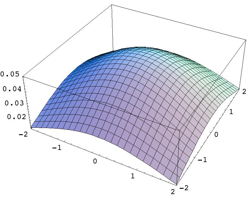 |
| Figure 4 - Model PRF kernel (Eq. 2) for WISE band-3. The area (or volume) under the function is unity. The x and y axes are in detector pixel units. The mesh shows the contribution of the flux at some point (x, y) as measured by a pixel centered at (0,0) and covering -0.5 to 0.5 along each axis. Click on plot to enlarge. |
The pixelated model PRF kernel (normalized to unity) for band-4 using the above construction is as follows. This is based on integrating the kernel shown in Figure 5 over a 9x9 detector pixel grid centered at (0, 0).
0.0946975  0.118335  0.0946975
0.1183350  0.147872  0.1183350
0.0946975  0.118335  0.0946975
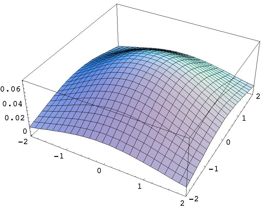 |
| Figure 5 - Model PRF kernel (Eq. 2) for WISE band-4. The area (or volume) under the function is unity. The x and y axes are in detector pixel units. The mesh shows the contribution of the flux at some point (x, y) as measured by a pixel centered at (0,0) and covering -0.5 to 0.5 along each axis. Note, the native pixel size for band-4 is 5.5 arcsec, compared to 2.75 arcsec for the other bands. Click on plot to enlarge. |
Figure 6 shows the effect of varying the width of the smoothing kernel on the coverage distribution output by the simulator. Coverage depths that are previously zero or low in the no smoothing case become effectively non-zero or larger after kernel smoothing. Note, "no smoothing" is equivalent to using a kernel which spans effectively one detector pixel - the most compact kernel possible.
So, why are there no coverage depths <5 in the kernel smoothing cases in Figure 6? Put another way, why does kernel smoothing result in relatively larger coverage depths at locations that were previously lower (i.e., with no kernel smoothing)?
The main thing to keep in mind is that in the kernel smoothing case, the effective depth-of-coverage at a location on the sky is given by the sum of weights contributed by all unit-normalized overlapping PRFs from all the good pixels.
Here's a simple (scaled down) example of what happens in practice. Suppose we have _no_ kernel smoothing, four overlapping frames, and one of the frames contains a bad pixel. At the sky location containing that one bad pixel in the stack, the coverage would be three. Now let's introduce kernel smoothing. At the location of that bad pixel, we will have (non-zero) information collected from that location on the sky by neighboring good pixels. I.e., the PRFs of the neighboring good pixels have wings that overlap at that location. So, given the four overlapping frames, the total coverage at that "bad" location is no longer 3, but effectively >3 - the exact value given by the sum of all the PRF weights from "good" neighbors that overlap at that location.
So, information from a sky location covered by a bad hardware pixel will be "collected" by the PRF "wings" of good neighbors to give in effect, a non-zero depth-of-coverage at that location on the sky.
The dependence in Figure 6 can thus be explained by having more good pixels than bad pixels in the array (thank goodness for that!), and good-pixel information "leaking" into bad pixel regions. When you sum many frames in a stack, the "low" coverage regions with say <~6 (before smoothing) get "higher" effective coverage after smoothing. Note that there are regions in the kernel smoothing case that still have coverages <5. These fractions are tiny, and are eliminated by the simulator since it only reports coverage fractions to 4 significant figures.
Even if you are undersampled with say a detector pixel spanning up to one FWHM of the PSF beam, the sky at the location of a bad pixel will still be covered by the non-negligible PRF wings of neighboring good pixels. In the limit of dense over-sampling of the PSF (much above Nyquist), the gain in effective coverage is maximized, and especially more so if the bad pixels are distributed as single isolated pixels. The effective coverage will gradually degrade as the bad pixels become more clumped. This is because a significant fraction would then be shielded from the PRF tails of good pixels that exist only around the clump peripheries and beyond.
The above discussion does not mean that bad pixels can be completely mitigated by the smearing effect of the PRFs from good pixels. There is still a net loss of information when bad pixels are present. The effective coverage is slightly lowered at the sky location of good pixels that are next to bad ones. This is because the information (or coverage) loss at the location of bad pixels is also smeared out, i.e., by the fact that their PRFs are "missing". The end result is reduced depth-of-coverage on average and hence achievable sensitivity.
Note that smearing by the PRF
itself also leads to a reduced point source sensitivity.
This is brought about by an increase in the equivalent number of
"noise pixels" contributing to a point source flux measurement.
The RMS sensitivity scales as √Np.
In other words, the wider a PRF (or the more sampled it is), the more it admits
potentially noisy pixels whose cumulative effect is to increase the total noise.
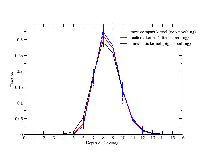 |
| Figure 6 - Dependence of the distribution in coverage depth on the width of the PRF smoothing kernel. These are based on the fpa143 (band-2) mask. The realistic kernel case (red lines) assumes the kernel in Figure 3. Click on plot to enlarge. |