 |
Coverage Simulations for Flight Arrays and Spares |
 |
I. Introduction
Below we summarize simulations of the achievable depth-of-coverage generated
using bad-pixel masks from all flight-worthy arrays (and spares). The objective
is to assess the impact of bad pixels on the WISE sky depth-of-coverage
and hence sensitivity.
It's important to note that these
simulations are based on: (i) candidate arrays from ground
testing, and (ii) the most realistic mission design parameters available
at the time of writing. Things may well change once in flight.
II. Assumptions
- The bad-pixel masks were constructed using
the criteria outlined here.
- Simulations only pertain to the ecliptic equator. Frame convergence
off the equator will increase the depth-of-coverage. Therefore,
the results below yield the "lowest" possible
coverages achievable with WISE.
- Each simulation spans an area ~46.9 x 93.8 arcmin. This effectively
represents ~0.7%
of the sky centered on the ecliptic equator when
compared to the full ecliptic latitude range
[-90° ≤ b ≤ 90°].
- Random orbit-to-orbit frame phasing was assumed in the in-scan direction, i.e.,
for each new orbit, the in-scan location of the starting (first) frame is some
random offset relative to the starting frame in the previous
orbit.
- A frame-to-frame in-scan step size of 41.538 arcmin (based on a 5720
sec orbital period and 11 sec frame cadence).
- An orbit-to-orbit cross-stepping of +30.65 (in the forward direction)
arcmin followed by -22.15 arcmin (in the reverse direction). This
gives the maximum desired coverage at the ecliptic after 15 orbits
(~1 day), given (approximately) the natural precession rate.
- Data loss due to SAA avoidence was simulated by dropping four
consecutive orbits starting at the fourth orbit out of every 15.
- At the time of writing, the orientation of arrays (in-scan versus
cross-scan) is unknown. Therefore, two sets of simulations,
orthogonal to each other were performed.
- Simple image-mask combination algorithms are assumed for estimating
coverages. For example, there is no sub-pixel interpolation onto a
coadd grid. The coverage at the location of a coadd pixel, contributed by
all frames in a stack, is the sum of all overlapping input pixel
values at that location.
- To better represent the impact of smoothing by
an interpolation kernel (as will be used in WISE Atlas image generation),
we assumed approximate Point Response Functions (PRFs) from optical
modelling and convolved these with the masks for each respective
band. When used in the coverage simulations, this results in an
effective coverage-depth as represented by the smearing
of "good" pixel information on the sky, and not the depth
expected by summing the number of overlapping physical detector pixels.
These two measures however turn out to be very close given the compact
nature of the WISE PRFs.
A description of interpolation kernel smoothing, assumptions, and impacts
can be found in:
Use of Smoothing Kernels.
- Other details on the method used by the core simulation software are
outlined in Section II.2 of
Coverage
Simulations for WISE Detector Acceptance Testing. The coverage maps
in this previous work correspond to one realization of a simulated 15 orbit
scenario - essentially a single execution of the software. To get a
handle on the dispersion in the fraction of pixels with a given coverage, we
executed 100 independent realizations of the software for each orientation.
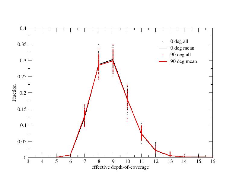
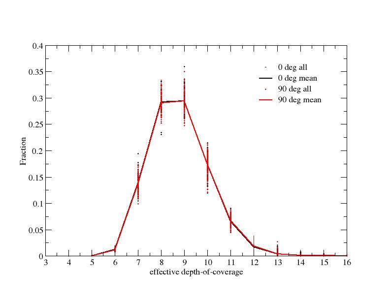
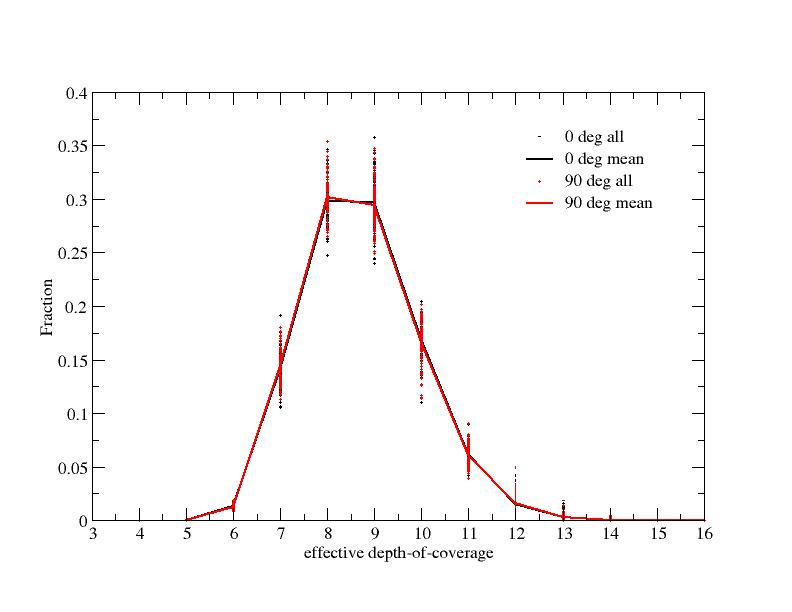
III. Results
The following table summarizes the FPA devices, bad-pixel status, and
their impact on the acheivable depth-of-coverage.
Note: FPAs 26 and 37 were recently reflowed (or repressed) to reduce the
number of bad pixels - mainly those pixels with excessive dark current.
| Band |
Flight FPA1 |
%Bad Pix.2 |
%Cov ≤ 83 |
Spare FPA4 |
%Bad Pix. |
%Cov ≤ 8 |
| 1 |
136: M, F |
1.201 |
41.54; C, D |
143: ?, ? |
2.823 |
44.82; C, D |
| 2 |
147: M, F |
3.238 |
45.29; C, D |
143 |
2.832 |
44.32; C, D |
| 3 |
26: M, F |
0.151 |
41.08; C, D |
31: ?, ? |
0.247 |
41.04; C, D |
| 4 |
37: M, F |
0.247 |
41.51; C, D |
31 |
0.875 |
41.37; C, D |
Notes:
- Flight array as selected by Project Office according to performance,
stability, and bad-pixel count. Click on a
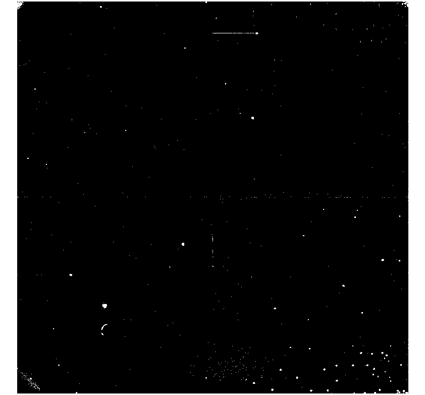
"M" for a JPEG of the bad-pixel mask.
Bad pixels are shown in white. Click on a "F"
to download the mask in FITS format.
- Approximate percentage of bad-pixels in the active region of each array,
i.e., excluding the four-pixel reference border.
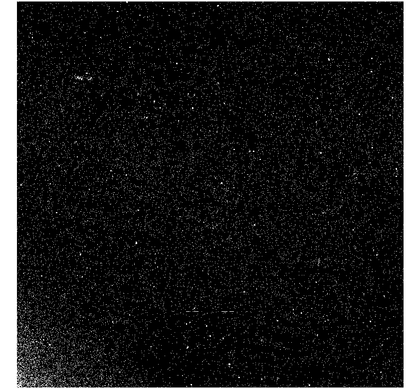
- The percentage of area on the ecliptic equator expected to have
coverage-depths of eight or less. Click on a
"C" for JPEGs of the coverage maps, and on a
"D" for the full coverage-depth
distribution at two orientations. The range in the coverage maps
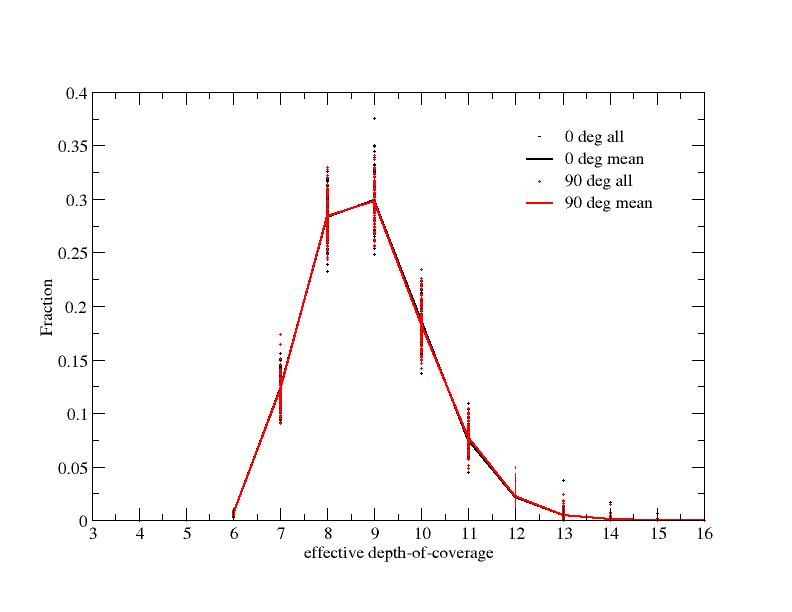
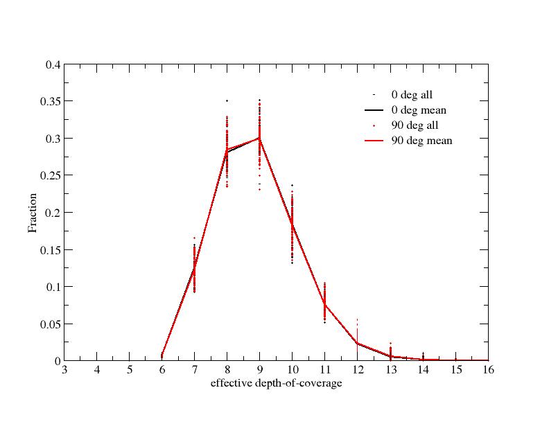
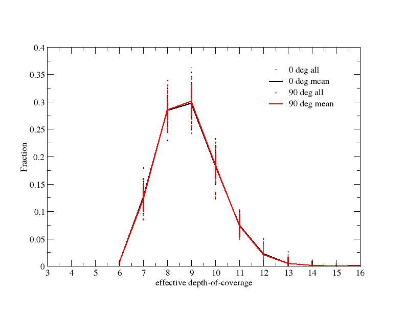
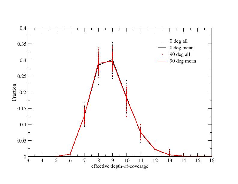
represent: 5 (darkest) to 13 (white) throughout. The fractions in
the coverage distributions are normalized such that they sum to unity.
Dots in the coverage distributions represent the 100 individual realizations
(simulation runs), and the lines go through the mean fractions from all
realizations. The cumulative coverage fractions in columns 4 and 7 were
computed by summing the mean fractions across all realizations. The random
error in these fractions is ~ ±9% (1-sigma) throughout.
- "Spare" or back-up flight array. The next two columns show
the same diagnostics for these spare arrays. Note: even though
bands 1 & 2, and bands 3 & 4 share the same spare arrays,
the coverage simulations are different for each band. This is
because they depend on the specific smoothing kernel for that band.
Last update - 20 February 2008
F. Masci, R. Cutri, T. Conrow - IPAC