Coverage Simulations for Band 2 Candidate Array (fpa141)

I. Introduction

We present simulated depth-of-coverage maps using bad-pixel masks constructed from a WISE band-2 (4.7μm) candidate array. This is referred to as detector "FPA141" in the test suite. The objective is to support detector acceptance testing by assessing the impact of bad pixels on the WISE sky depth-of-coverage.

The simulations below are a continuation of those presented for bands 3 and 4 (Si:As arrays): Coverage Simulations for WISE Detector Acceptance Testing. Below we adopt the same assumptions, methodology and software as presented therein, but with a slight improvement in the analysis method.

1. Inputs

The main input is a bad pixel mask image provided by the WISE Science Project Office. This was recieved as a 1024x1024 FITS image with bad pixels denoted with a value "1", and good pixels denoted with value "0". We further included the 4-pixel wide "reference pixel" border around this mask flagged with 1's. This is an inactive region of the array whose readout will be used for DC-offset calibration.

For the FPA141 candidate array, bad pixels were identified using the following criteria:

Dark currents exceeding 5 e-/sec (denoted "bad dark").
Read noise as measured from 8-SUR darks of > 30 e- (denoted "bad noise").
Low responsive pixels with < 0.5 or > 1.3 in flat normalized to unity using mean (denoted "bad flat").
Pixels that reach 65535 ADU anywhere in their 8-sample ramps (denoted "bad sat").
Pixels subject to "Inter-Pixel Capacitance" (IPC) effects - flagged as the four nearest neighbors to pixels with dark exceeding 300 e-/sec (denoted "bad IPC").

For more details, please contact the WISE Science Project Office at JPL.

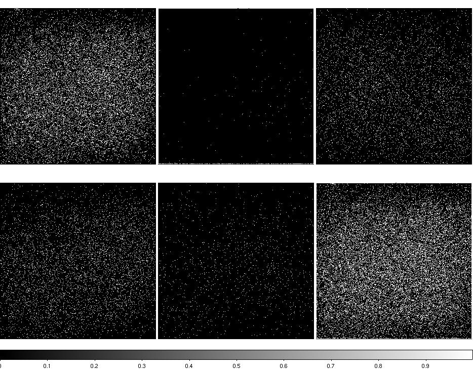
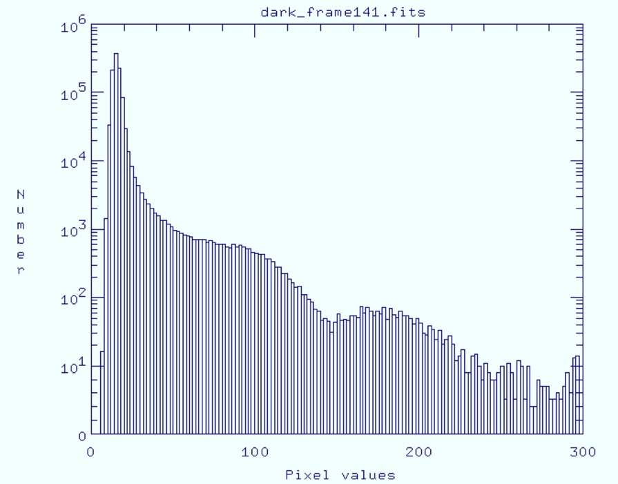
With the above noted criteria, ~22.1% of pixels in FPA141 (in the active region only) are declared as bad. The dominant effect (>16%) is excessive dark current. The FPA141 masks, corresponding to each of the above five criteria are shown in Figure 1. The image at bottom right is the mask containing bad pixels flagged using all criteria. Figure 2 shows a histogram of the dark frame used in the analysis.

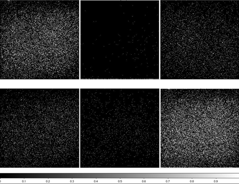Figure 1 - Bad-pixel masks created using criteria in Section I.1. Top row (left to right): "bad dark"; "bad flat"; "bad noise". Bottom row (left to right): "bad IPC"; "bad sat"; "total bad pixels".

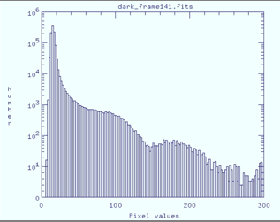Figure 2 - Histogram of dark pixel values (e-/sec) for test array FPA141.

II. Methodology

1. Assumptions

The simulations below make use of realistic mission design parameters available at the time of writing. It's important to note that these are only approximate. Here are the main assumptions:

Simulations only pertain to the ecliptic equator. Frame convergence off the equator will increase the depth-of-coverage. Therefore, the results below will yield the "lowest" possible coverages achievable with WISE.
Random orbit-to-orbit frame phasing was assumed in the in-scan direction, i.e., for each new orbit, the in-scan location of the starting (first) frame is some random offset relative to the starting frame in the previous orbit.
A frame-to-frame in-scan step size of 41.538 arcmin (based on a 5720 sec orbital period and 11 sec frame cadence).
An orbit-to-orbit cross-stepping of +30.65 (in the forward direction) arcmin followed by -22.15 arcmin (in the reverse direction). This gives the maximum desired coverage at the ecliptic after 15 orbits (~1 day), given (approximately) the natural precession rate.
Data loss due to SAA avoidence was simulated by dropping four consecutive orbits starting at the fourth orbit out of every 15.
At the time of writing, the orientation of arrays (in-scan versus cross-scan) is unknown. Therefore, two sets of simulations, orthogonal to each other were performed.
Simple image-mask combination algorithms are assumed for estimating coverages. For example, there is no sub-pixel interpolation onto a coadd grid. The coverage at the location of a coadd pixel, contributed by all frames in a stack, is the sum of all overlapping input pixel values at that location. Also, the resolution in the output coverage-depth statistics is 1 pixel. These coverage estimates should be very close (to first order) to those achievable with a more sophisicated coaddition process, e.g., one that uses kernel interpolation onto a coadd grid.

2. Procedure

The method used by the core simulation software is outlined in Section II.2 of Coverage Simulations for WISE Detector Acceptance Testing. The coverage maps in this previous work correspond to one realization of a simulated 15 orbit scenario - essentially a single execution of the software. To get a handle on the dispersion in the fraction of pixels with a given coverage, we executed 100 independent realizations of the software.

a. Test Sequence

We performed three separate simulations, each consisting of 100 (15-orbit) coverage realizations, corresponding to three separate bad-pixel masks:

Default FPA141 mask derived from all bad-pixel criteria outlined in Section I.1.

Same FPA141 mask, but now convolved with an interpolation kernel. The interpolation kernel is represented by the best available estimate of the PRF as deduced from optical characterization. An interpolation kernel will be used for optimal WISE Atlas image generation. The interpolation kernel has the effect of smearing (or smoothing) "bad" as well as "good" pixel information across the sky. Since source detection will primarily occur off the WISE Atlas (coadd) images, the impact of kernel smoothing on effective converage depth in the presence of bad pixels must be deduced. This will enable a more reliable estimate of sensitivity in the long run. A description of interpolation kernel smoothing, assumptions, and impacts can be found in: Use of Smoothing Kernals.

For comparison, a hypothetical "perfect" detector mask with no bad pixels, but with the 4-pixel wide "reference pixel" border included.

III. Test results

A summary of the three simulation runs outlined in Section II.2.a with links to image masks and coverage maps in FITS format is given in Table 1.

**Table 1 - Coverage Simulation Test Summary for HgCdTe detector FPA141**
Test Run	FITS Mask¹	FITS Coverage Map²	Rotation (deg)
1	bad_pix_tot141	bad_pix_tot141_cov0	0
	bad_pix_tot141	bad_pix_tot141_cov90	90
2	bad_pix_tot141_smooth	bad_pix_tot141_smooth_cov0	0
	bad_pix_tot141_smooth	bad_pix_tot141_smooth_cov90	90
3	perfect_mask	perfect_cov	0 and 90

Notes to Table 1

Click on this column to download the mask image in gzip'd FITS format. Default mask used in Test 1 was provided by project office and a 4-pixel wide reference border was included by us. The mask used in Test 2 includes more bad pixels from kernel smoothing - see Section II.2.a
Click on this column to download the simulated coverage map in gzip'd FITS format. A map here represents that which falls closest to the mean coverage fractions computed over 100 realizations (executions) - see Figures 4, 6 and 8 for histograms.

For each of the test runs outlined in Section II.2.a, we present below mean coverage fractions, maps and histograms computed from the 100 realizations. At a specific depth-of-coverage, these statistics represent the mean fraction of pixels within a simulated 2048x1024 central region. The mean is computed over all realizations. The coverage maps represent those whose coverage fractions fall closest to the mean fractions at the respective coverages.

1. Test Run #1 (Default Mask)

cov.  mean fraction (0 degrees)
1   0.00028095
2   0.00269352
3   0.01501135
4   0.05342559
5   0.12717760
6   0.20711752
7   0.23365784
8   0.18587726
9   0.10747607
10  0.04660579
11  0.01552126
12  0.00400829
13  0.00080187
14  0.00016247
15  0.00008254
16  0.00009998

cov.  mean fraction (90 degrees)
1   0.00018898
2   0.00191286
3   0.01227612
4   0.04846052
5   0.12448507
6   0.21257476
7   0.24403050
8   0.19138428
9   0.10563242
10  0.04248395
11  0.01287307
12  0.00300378
13  0.00053596
14  0.00011322
15  0.00004444


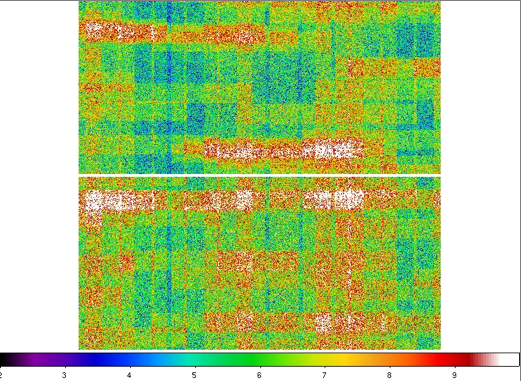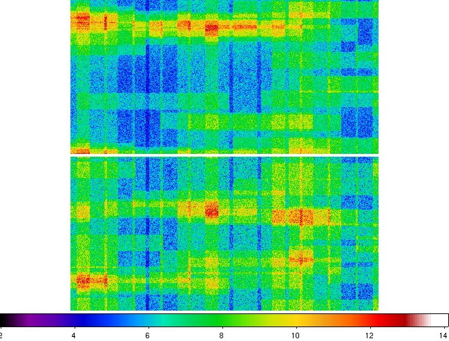
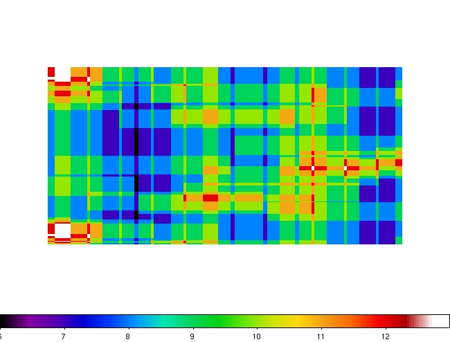
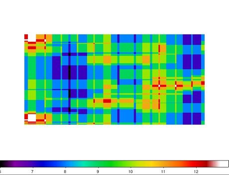
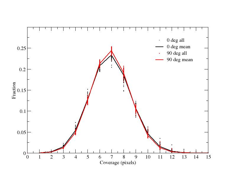
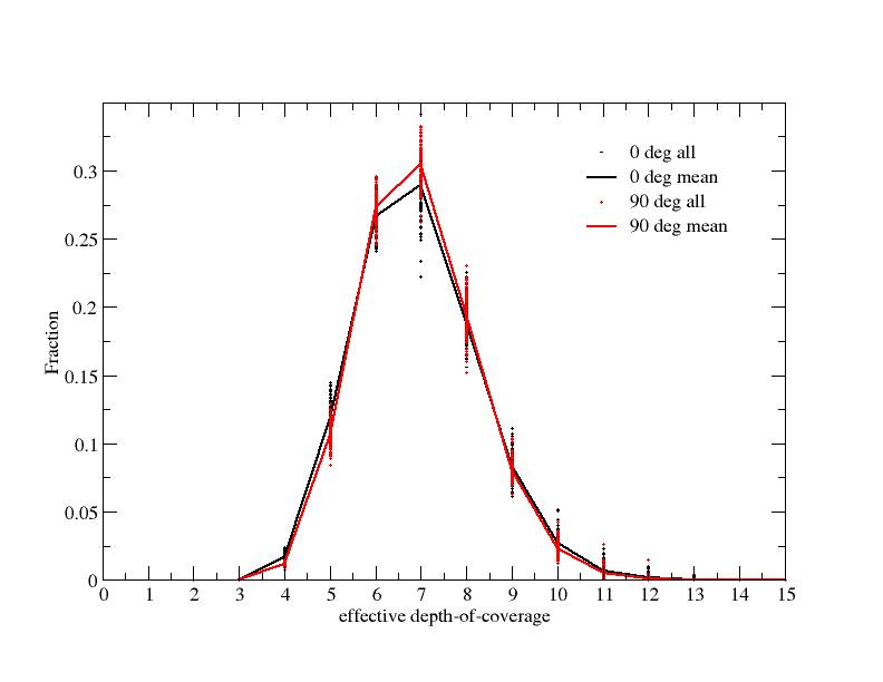
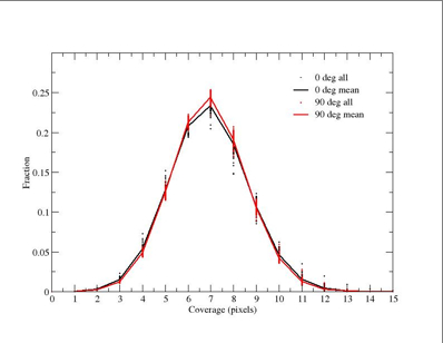
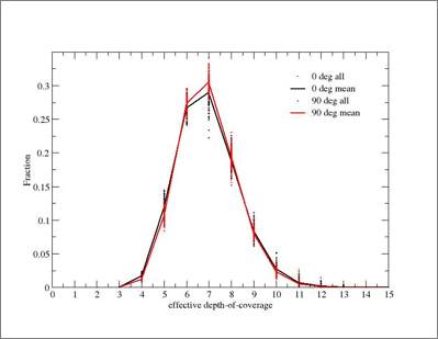
Figure 3 - Coverage maps for Test 1: top = 0 degrees; bottom = 90 degrees.	Figure 4 - Coverage distributions for Test 1.
Left: false color JPEG images of coverage maps for Test 1. The color bar at the bottom corresponds to the approximate coverage in pixels. The approximate range shown is ~3.5 (blue) to 10 (white). Right: corresponding coverage distribution with fractions normalized to unity. Dots represent the 100 individual realizations. The lines go through the mean fractions from all realizations. Click on thumbnails to see full-size JPEG maps.

Summary

For the default FPA141 mask that uses all the bad-pixel criteria, ~64% of the area (the mean at 0 or 90 degrees) has fewer than 8 coverages. Approximately 1.4%-1.7% has fewer than 4 coverages. But note, since the reported statistics are limited to a resolution of 1 detector pixel in coverage depth, the percentage with effective depths < 4 can be closer to ~5%;
As a reminder, a minimum coverage of 4 over at least 95% of the whole sky is the mission requirement. But note, our simulation area effectively represents ~0.7% of the sky centered on the ecliptic equator when compared to the full ecliptic latitude range [-90 to 90 degrees]. 8 coverages is used to define the baseline sensitivity requirement;
The mode coverage is ~7. The RMS scatter about the mean fraction at this value is ~ +/-1.8% (both 0 and 90 degrees) and is representative at other coverages;
For 100 realizations, the standard error in the mean fractions quoted above is of order RMS/sqrt(100) ~ +/-0.18%;

2. Test Run #2 (with Kernal Smoothing)

cov.  mean fraction (0 degrees)
3   0.00050197
4   0.01632704
5   0.11854209
6   0.26657947
7   0.28923915
8   0.18883699
9   0.08385611
10  0.02738140
11  0.00702859
12  0.00141391
13  0.00024879
14  0.00004444

cov.  mean fraction (90 degrees)
3   0.00025997
4   0.01159792
5   0.10608218 
6   0.27266377
7   0.30500977
8   0.19495896
9   0.08004259
10  0.02309086
11  0.00512552
12  0.00093691
13  0.00016984
14  0.00004166
15  0.00001999


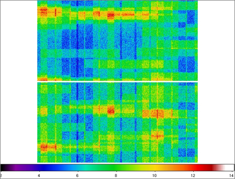
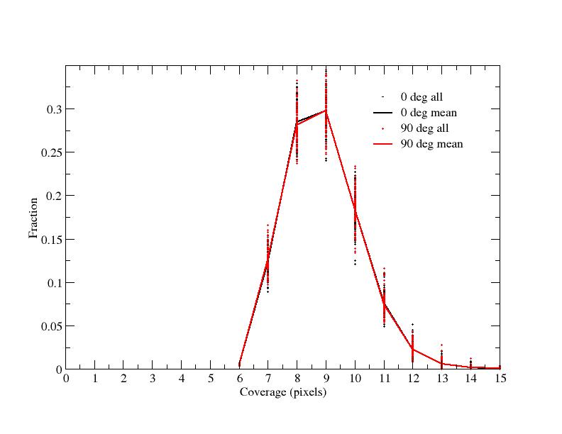
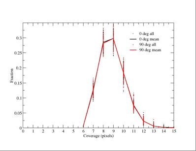
Figure 5 - Coverage maps for Test 2: top = 0 degrees; bottom = 90 degrees.	Figure 6 - Coverage distributions for Test 2.
Left: false color JPEG images of coverage maps for Test 2. The color bar at the bottom corresponds to the approximate coverage in pixels. The approximate range shown is 4 (dark blue) to 12.5 (red). Right: corresponding coverage distribution with fractions normalized to unity. Dots represent the 100 individual realizations. The lines go through the mean fractions from all realizations. Click on thumbnails to see full-size JPEG maps.

Summary

For the same FPA141 bad-pixel mask convolved with a model interpolation kernel, ~70% of the area (the mean at 0 or 90 degrees) has fewer than 8 coverages. Approximately 1.1% - 1.7% has fewer than 4 coverages;
The mode coverage is ~7. The RMS scatter about the mean fraction at this value is ~ +/-2.6% (both 0 and 90 degrees) and approximately representative at other coverages;
For 100 realizations, the standard error in the mean fractions quoted above is of order RMS/sqrt(100) ~ +/-0.26%;

3. Test Run #3 (Perfect Mask)

cov.  mean fraction
6   0.00524177
7   0.12215591
8   0.28407260
9   0.29720000
10  0.18370580
11  0.07606465
12  0.02320443
13  0.00611416
14  0.00151106
15  0.00052980
16  0.00019976


Figure 7 - Coverage map for Test 3.	Figure 8 - Coverage distributions for Test 3.
Left: false color JPEG images of coverage maps for Test 3. The color bar at the bottom corresponds to the approximate coverage in pixels. The approximate range shown is 6 (black) to 13 (white). Right: corresponding coverage distribution with fractions normalized to unity. Dots represent the 100 individual realizations. The lines go through the mean fractions over all realizations. Click on thumbnails to see full-size JPEG maps.

Summary

For the perfect hypothetical scenario (no masked pixels, only a 4-pixel wide reference border), we expect approximately 12% of the area to have fewer than 8 coverages. No regions have coverages under 4;
Note, this example is purely for comparison purposes;
The mode coverage is ~9. The RMS scatter about the mean fraction at this value is about +/- 2.2%;
For 100 realizations, the standard error in the mean fractions quoted above is of order RMS/sqrt(100) ~ +/-0.22%;

IV. Conclusions

Given the default FPA141 (band-2) bad-pixel mask, up to 5% of an area on the ecliptic equator will have fewer than 4 coverages, and ~64% will have fewer than 8 coverages (see Figure 4). The simulated area effectively represents ~0.7% of the sky.
With inclusion of smoothing from an interpolation kernel as represented by a model PRF fit, the fraction with fewer than 4 coverages drops to ~1.1 - 1.7%, while ~70% will have few than 8 coverages (see Figure 6). For your information, interpolation kernels will be used for optimal Atlas image generation.
The reason for these slight (but significant) drops in areas with low-coverage when kernel smoothing is present is due to a "smearing" of good pixel information into adjacent bad pixels (mainly because there are more good pixels than bad ones). This effectively increases the depth-of-coverage at the locations of bad pixels on the sky.
The impact of an interpolation kernel on increasing the effective depth-of-coverage at bad pixels is maximized if the bad pixels are more-or-less randomly distributed as single isolated pixels. If the same number of bad pixels were in larger concentrations, a large fraction would be shielded by the PRF tails of good pixels and thus, the average depth-of-coverage is expected to decrease.
Note: the above does not mean that bad pixels can be completely mitigated by the smearing effect of the PRF. There is still a net loss of information when bad pixels are present in that the effective coverage is slightly lowered at the location of good pixels that are next to bad ones. Also, smearing by the PRF itself results in reduced point source sensitivity by an amount proportional to the square root of the equivalent number of "noise pixels" contributing to a flux measurement. The number of noise pixels is characteristic of the PRF. For more details on kernel smoothing and noise pixels, see: Use of Smoothing Kernals.

Last update - 27 June 2007
F. Masci, R. Cutri, T. Conrow - IPAC