IV. WISE Data Processing

5. Multiframe Pipeline

c. WISE Photometry System (WPHOT)

Contents

1. Memory Optimization
2. Coordinate Translation
3. Local Background Estimation
4. Bright Stars

1. The Point Spread Function
2. WPRO Output Parameters
3. WPRO Magnitude Upper Limits
4. Saturation and Latent Fractions
5. Frame Detection and Flux Repeatability Statistics
6. Variability and Flagging

1. Special Inputs
2. Circular Apertures
3. Output
4. Confusion and Warning Flags
5. Magnitude Upper Limits

WPHOT is designed to perform the source position and flux characterization step associated with each of the three stages of source extraction during pipeline processing (single-frame, single-epoch 4-band frameset, and final multi-frame coadd stage). The characterization is based on an input list of source candidate positions produced by the source detection module, MDET, using a detection algorithm which makes use of the data at all bands simultaneously.

Since the majority of sources detected by WISE are expected to be spatially unresolved, the optimal approach for source characterization involves profile-fitting photometry (WPRO). Profile-fitting is our primary method of flux estimation -- it gives the best results for the majority (i.e., the fainter) sources, handles PSF variations and masked pixels in an optimal fashion, and extends the dynamic range for bright sources well into the saturated regime.

Just as with the detection step, profile-fitting is carried out using the data from all bands simultaneously. The advantages of simultaneous multiband extraction are:

1. Increased sensitivity to weak sources due to the fact that detection is based on the stack of images at all bands.


2. No separate bandmerging step is required, thus avoiding the ambiguities which can occur when trying to associate sources in different bands in the presence of confusion.


3. The higher resolution data at the shorter wavelengths can guide the extraction at the longer wavelengths where the resolution is poorer.

The multiband estimation process represents a departure from the traditional procedure, employed in such software packages as DAOPHOT (Stetson 1987) and SExtractor (Bertin & Arnouts 1996), in which detection and characterization are carried out one band at a time. Another motivation for developing new source extraction algorithms is that currently available packages operate on a single regularly-sampled image rather than a set of dithered images. The procedures employed in MDET and WPHOT are optimized for the latter case.

Since the majority of sources are unresolved, the profile-fitted flux represents our best estimate in most cases. For extended sources (one indicator of which is an elevated chi squared value), an aperture flux should be used instead. Therefore, in addition to profile-fitting photometry, WPHOT includes an system (WAPPco) that employs circular apertures to characterize the integrated flux and `curve-of-growth' of point sources as measured in the co-added images. Those sources that are within close proximity to a 2MASS XSC (galaxy) are further characterized using an elliptical aperture derived from the 2MASS XSC.

Figure 1 - WPHOT overview flowchart

ii. WPHOT Executive

1. Memory Optimization

The compromise solution is to break the large co-add 'footprint' into a smaller pieces, processing each piece separately. The cost is i/o overhead from reading in the frames multiple times, once for each grid piece. An example of a 3x3 divided footprint is shown in the diagram; a savings in memory load of nearly 50% is possible with such a gridding. The optical grid configuration, balancing run-time and memory usage is found to be 5x5.

Figure 2 - WISE W1 co-add image, 4095x4095 pixels. The field has been divided into 3x3 pieces, thus reducing each piece to 1365 coadd pixels, or 683 frame pixels. A memory reduction of 45% is realized with this case. A small amount of overlap is needed to guarantee full processing coverage near division edges.

The basic algorithm steps follow from the Co-add 'footprint' divided into NxM pieces with enough overlap to take into account spacecraft rotation (w/ respect to equatorial north) and minimum border tolerance for background and source flux estimage; each piece is processed separately as follows:

• sub-frames allocated; frame pieces loaded into sub-frames


• sub-MDET table allocated and loaded into memory


• source X,Y positions loaded into memory


• source background information computed and loaded into memory (local background, RMS and "confusion" metric)


• WPRO executed w/ sub-frames, sub-MDET, XY position and background information as input


• duplicate sources (from division edge overlaps) removed using fast algorithm


• WPRO extractions loaded into master extraction table

2. Coordinate Translation

3. Local Background Estimation

• Standard annulus radii: 50 to 70 arcsec (W1, W2, W3, W4)

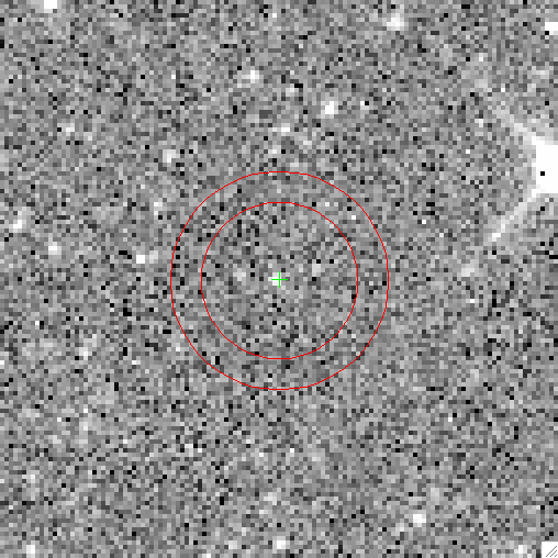
The local background is determined from the pixel value distribution within a circular annulus centered on the source MDETposition. The source background, b_λ and σ^2_bann, representing the local ``sky'' background level and its uncertainty, are estimated from the trimmed average of the pixel value distribution, where the trimming is driven by the 50% (median) and 16% (lower 1-σ) histogram shape and thus robust to contamining sources in the annulus (whose pixel values reside on the positive side of histogram median); see Figure 3 for illustration.

The formal background error, or sigma in the mean, is derived from the the error propagation that follows the instrument characteristics and the noise model that is tracked by AWAIC and passed to on to WPHOT. With this noise model, the formal uncertainty in the background sky level is

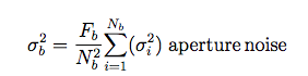(Eq. 1)

where N_b is the number of pixels in the annulus and σ_i is the measurement uncertainty for detector/frame pixel i, and F_b is the correlation factor that is appropriate to the images being measured (for WISE frames, the factor is unity, and for co-adds it ranges between 30 and 225, W1 to W4, respectively).

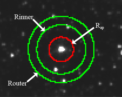Figure 3 -- parameters: standard aperture (red) and local background annulus (green).

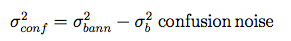
The formal background uncertainty is not sensitive to confusion noise that may be present in the aperture or annulus. It therefore requires a correction to account for any stellar crowding or confusion noise. A reasonable proxy to the total noise comes from the annulus background uncertainty, σ^2_bann. We therefore make the assumption that the confusion noise is the difference between the total noise in the annulus and the formal (Poisson) noise in the aperture:

(Eq. 2)

For most of the sky, the confusion noise term is zero or negligible in value, but for the Galactic Plane where stellar crowding is an important concern, the confusion noise term may be appreciable.

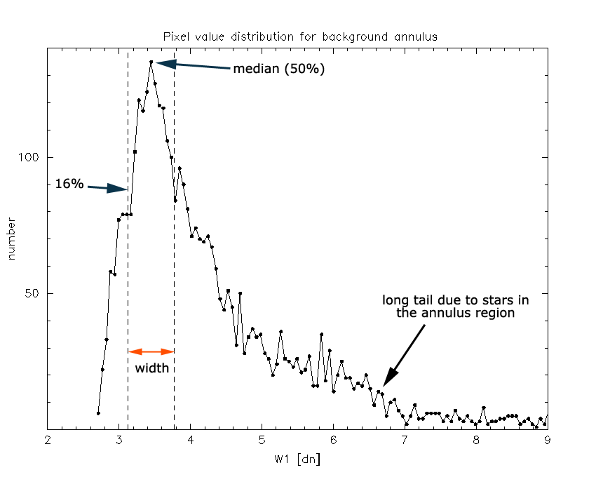Figure 4 - Example of a background annulus and its pixel value distribution (right panel).	Figure 5- The local background is estimated from trimmed average of the pixel value distribution in the local background annulus. Using iterative convergence, the trimming is based on the left side of the histogram median, where the width is gauged from the 16% quartile to the 50% (median).

Choosing the optimal size for the annulus is an important consideration toward accurate photometry. The annulus must be large enough to avoid the influence of the point spread function and to minimize the Poisson component of the sky pixels (see equation below). On the other, it must also be small enough to represent the ``local'' sky value (that is to say, the fluctuations that are present in the aperture should be of similar amplitude in the annulus). Moreover, in order to accommodate the possibility of the source being fuzzy galaxy, the annulus should extend beyond the size expected for most galaxies in the sky.

Consider what was done with 2MASS background estimation. For standard 2MASS point source photometry, the annulus that was used: R_inner = 14 arcsec, R_outer = 20 arcsec, with 2 arcsec pixels that translates to 160 pixels in the annulus. The 2MASS beam is about 2.5 arcsec, so R_inner is ~6x the FWHM. For the combined calibration fields, 2MASS used a larger annulus, 24 - 30 arcsec in size, or roughly ~10x the FWHM. The standard calibration aperture for IRAC is 12 arcsec, and the annulus is 14.4 - 20 arcsec, which compared to the 2 arcsec beam is ~7 - 10x the FWHM.

For WISE, the FWHM=6 arcsec for the short channels, and so using 2MASS/IRAC as a guide, the inner radius would be ~40 - 50 arcsec (80 - 100 arcsec for WISE-4); with 2.75 arcsec pixels, that translates to R_inner ~ 15 - 18 pixels. For the width, using a similar area as the 2MASS/IRAC annulus, then R_outer ~ 19 pixels. Since that is a relatively thin aperture, subject to pixelization effects, it would be better to extend it to a width of 4 - 5 pixels, or R_outer = 20 - 22. Consequently, the adopted annulus for WISE point sources is: 50 - 70 arcsec (for all four bands), corresponding to 18-25 pixel radius in W1, W2, W3, and 9 to 13 pixels for W4. This setting is constrained by the W4 beam.

• w?sky : mean frame sky background in DN units
  
• w?sigsk : the formal uncertainty in the background sky level in DN units (Eq. 1)
  
• w?conf : estimated confusion noise in DN units (Eq. 2)

4. Bright Stars

iii. Profile fitting photometry (WPRO)

The purpose of this step is to make a maximum likelihood estimate of the source position and the set of fluxes at the four wavelengths for each source candidate identified by the detection module MDET. The candidate source and its neighbors (i.e., adjacent candidates whose PSF responses overlap significantly with the primary candidate) are grouped into blends, and their parameters estimated simultaneously; this process is referred to as passive deblending, and is incorporated explicitly into the photometric measurement model. The critical distance for blend grouping is driven by the size of the PSF at the longest wavelength;  neighbors separated from the source in question by less than twice the nominal FWHM at W4 (i.e., 24 arcsec) are included in the initial blend group.

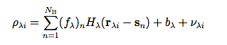
For a blend consisting of N_B components, the measurement model used in profile fitting is:

(Eq. 3)

where ρ_λi is the observed value of the ith pixel at 2-d sky location r_λi in the waveband denoted by subscript λ, s_n is a 2-d vector representing the location of the nth blend component, f_λn is the flux in the λth waveband, H_λ(r) is the PSF, b_λ is the local background, estimated in an annulus surrounding the candidate position, and ν_λi is the noise, assumed to be a spatially and spectrally uncorrelated zero-mean Gaussian random process with variance σ_λi².

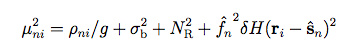
The latter quantity includes the various noise components in the error model and may be expressed as:

(Eq. 4)

where (σ_pix)_λi represents the uncertainty in the pixel value due to instrumental effects; it is calculated by module ICAL, and includes the effects of Poisson noise, read noise, and flat-fielding error. Also, (σ_conf)_λi represents the confusion noise, as defined by Eq. (2) above, and δH_λ(r) represents the PSF uncertainty which must be scaled by the source flux, f^{^}_λ. The "hat" symbol (^) over the latter quantity denotes an estimated value. Our best estimate prior to the profile fitting is the aperture flux; we follow this with a second iteration based on the profile-fitted flux from the first iteration.

The set of unknowns in the estimation process can be represented by an n_p-dimensional parameter vector, z, defined as:

(Eq. 5)

where N_λ represents the number of wavebands, and the number of unknowns is given by n_p = N_B(N_λ + 2).

The solution procedure is to maximize the conditional probability P(ρ|z,N_B) with respect to z, where:

(Eq. 6)

in which the summation over i is for all pixels within a predefined "fitting radius", r_fit, of the candidate source location. Pixels which are flagged as "bad," due to effects such as saturation and cosmic ray hits, are excluded from the solution. We normally set r_fit = 1.25 x FWHM, where the latter quantity represents the nominal FWHM of the PSF at the particular band, equal to 6, 6, 6, and 12 arcsec in bands W1 through W4, respectively. However, in the case of saturated stars, we set r_fit = max(2r_sat, 1.25xFWHM), where r_sat is the effective radius of the saturated core of the bright star, calculated by the MDET module.

The quality of the fit is then evaluated using the reduced chi squared, given by:

(Eq. 7)

where N_obs represents the total number of pixel values used in the solution.

Before proceeding further, the blend group is first examined to check for redundant components, i.e., those components which can be removed without an increase in χ_ν². Thus the final value of N_B can, in some cases, be less than the initial value defined above.

If χ_ν² ~ 1, the fit is regarded as satisfactory. However, if χ_ν² is larger than a critical value, (χ_ν²)_crit, or if the reduced chi squared for an individual band (denoted (χ_ν²)_λ) exceeds a related threshold, (where phi is the relative number of degrees of freedom of the single-band fit with respect to the multiband fit), then we consider that the source model has not satisfactorily reproduced the observed data. We then examine the hypothesis that the true intensity distribution involves additional point source components. In this procedure, referred to as active deblending, we successively add more source components (thereby increasing N_B) until either χ_ν² < (χ_ν²)_crit or else the blend number reaches a predefined limit, (N_B)_max, at which point we conclude that a model consisting of a few point sources is not consistent with the observations. For reasons of computational speed, we allow at most 1 extra component to be added via active deblending.

At each iteration of the active deblending procedure, the mechanism for adding a new source component is as follows:

1. Construct a source model consisting of N_B components in the locations estimated in the current solution, plus an additional component offset by (Δx, Δy) from the primary source.


2. At each location on a regularly-sampled grid of (Δx, Δy) in a rectangular region surrounding the primary source, obtain the maximum likelihood solution for the set of (N_B + 1) fluxes of this set of components.


3. Calculate the corresponding χ_ν² as a function of (Δx, Δy).


4. Find the minimum of χ_ν²; we now have a set of (N_B + 1) component locations which serve as a starting model for a full maximum likelihood solution (position and fluxes)

1. Chi squared test (overall and for individual bands) as above. This test determines whether the data (and single-band subsets of the data) are consistent with the model.


2. Require that the overall reduced chi squared decrease by at least a minimum amount, i.e. Δχ_ν² > (Δχ_ν²)_min. The difference in chi squared corresponds to a likelihood ratio, and thus indicates the extent to which a model with (N_B + 1) components is more likely than a model with N_B components.

The overall profile-fitting photometry procedure is illustrated by the flow chart in Figure 6; the active deblending procedure is contained within the blue dashed rectangular box. Active deblending is required for sources whose separation is less than 1.3 times the FWHM of the PSF at a given band, since this is the critical distance at which the detector can resolve neighboring sources.

Figure 6 - WPRO Flow Chart

When a satisfactory solution has been obtained, the uncertainties in the estimated parameters (position and fluxes) are obtained using:

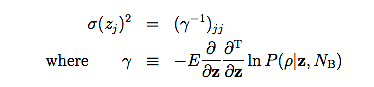(Eq. 8) (Eq. 9)

in which E is the expectation operator and T denotes transpose.

The way in which the above estimation procedure is implemented is that we start with the brightest source in the candidate list and estimate its parameters as above. We then proceed as follows:

1. Write out the source position and multiband fluxes associated with the candidate itself and with any actively-deblended source components (each of which is regarded as a separate source.


2. Discard the results for any passively-deblended components, i.e., those components corresponding to neighboring candidates in the MDET detection list---these candidates will be processed later.


3. Subtract the estimated contributions of the primary source (+ actively-deblended components) from the focal-plane images.

We then repeat the procedure for the next brightest candidate, and so on until the MDET candidate list is exhausted.

1. The Point Spread Function

Each PSF in the library represents an average over a focal-plane segment of width W_P, over which we approximate the PSF as locally isoplanatic. The driver for W_P is the Functional Requirement of at least 7% flux accuracy for an unsaturated source with SNR > 100. Our 9x9 subdivision of the focal plane exceeds this requirement by typically better than a factor of 4. We now discuss in detail the procedure used for PSF estimation in each focal-plane segment.

Estimation procedure

The measurement model for the PSF is then:

(Eq. 10)

where s_n is the location of the nth star in the segment. The origin of the coordinate system for the PSF image is defined to be at the star location.

The noise, ν_nj, is assumed to be an uncorrelated Gaussian random process for which

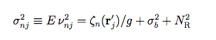(Eq. 11)

From the set of star images, we can make a maximum likelihood estimate of the PSF using:

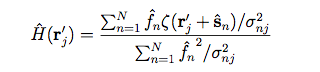(Eq. 12)

where f^{^}_n and s^{^}_n represent the estimated flux and position, respectively, of the nth star. For bright stars, an accurate flux estimate can be obtained via .

The source position s_n is estimated by adjusting the positional offset of the star image for maximum correlation with respect to a nominal starting PSF, H₀(r'), for which we used a theoretical form based on optical simulations. The estimation is accomplished by numerical minimization, with respect to s_n, of:

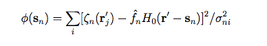(Eq. 13)

PSF uncertainty

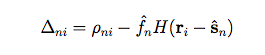(Eq. 14)

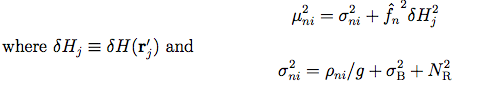
We model Δ_ni as a zero-mean Gaussian random process with variance

(Eq. 15)

where δH(r) represents the PSF uncertainty at offset r from the PSF origin; g and N_R represent the gain and read noise, respectively.

Suppose that the position (r_i - s_n) falls within the jth pixel on the grid used to represent the PSF, i.e.,

(Eq. 16)

(Eq. 17)

where (x'_j, y'_j) represent the components of r'_j, (ξ_n, η_n) represent the components of s_n, and δx, δy represent the sampling intervals of the PSF grid in the x and y directions, respectively.

Then:

(Eq. 18) (Eq. 19)

Thus the probability density of the set of local data residuals, Δ, conditioned on δH_j, is given by:

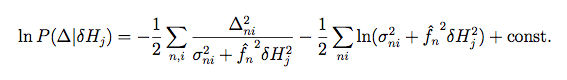(Eq. 20)

where the summations are over all n, i which satisfy Equations 16 and 17 for a given j.

This expression is maximized when:

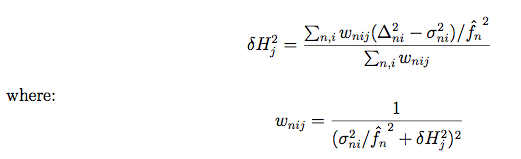(Eq. 21)   (Eq. 22)

Since δH_j is present on both sides of Equation 2), iterative solution is required. Convergence is rapid, however, and a single iteration suffices.

Steps involved in PSF generation

For each focal plane segment:

1. Locate all stars above a given flux threshold for the particular band.

2. Estimate PSF and its uncertainty using Equations 12 and 21.

3. For each individual star, examine the quality of its profile fit by evaluating χ_ν² using Equation 7.

4. List any stars for which χ_ν² exceeds a predefined threshold (~ 2); discard the star with the highest χ_ν²

5. Iterate from step 2 until all all remaining stars used in the PSF estimation have acceptable profile fits.

PSF generation from survey data

The PSFs and their corresponding uncertainty images, as used for the Preliminary Release, were generated one band at a time using the procedure described above. Candidate frames were selected from all scans between 01601a (by which time improved astrometry had been implemented) and 01751a. Initial frame selection was made by searching source detection tables for bright unsaturated stars, requiring SNR of at least 30 in the case of W4. This yielded 1028 candidate framesets. The W1 images were then visually examined to remove those images with obvious tracking problems (elongated images), high cosmic ray fluxes, highly crowded fields in the Galactic plane, structured backgrounds (e.g. nebulae), very bright stars saturating large areas of the array, and scattered moonlight. This selection process left 888 candidate framesets. The practical limit on the number frames that WPSFGEN can process at once is ~500, so another 300 framesets were removed by randomly rejecting framesets which had only one band four detection with W4SNR > 30. The final list of 484 frames provided 68749 unique sources with SNR > 100.

For bands W1-W3, PSFs were generated in 9x9 grids over the focal plane. Because of the relative scacity of bright stars in W4, a 5x5 grid was generated, and interpolated between adjacent PSFs to form a 9x9 grid. The following is aset of pseudocolor representations of the PSFs using a linear intensity scale, clipped at 60% of peak; the width of the field of view is 43.5 arcsec for W1-W3 and 87 arcsec for W4:

W1	W2	W3	W4
Figure 7 - WISE PSFs

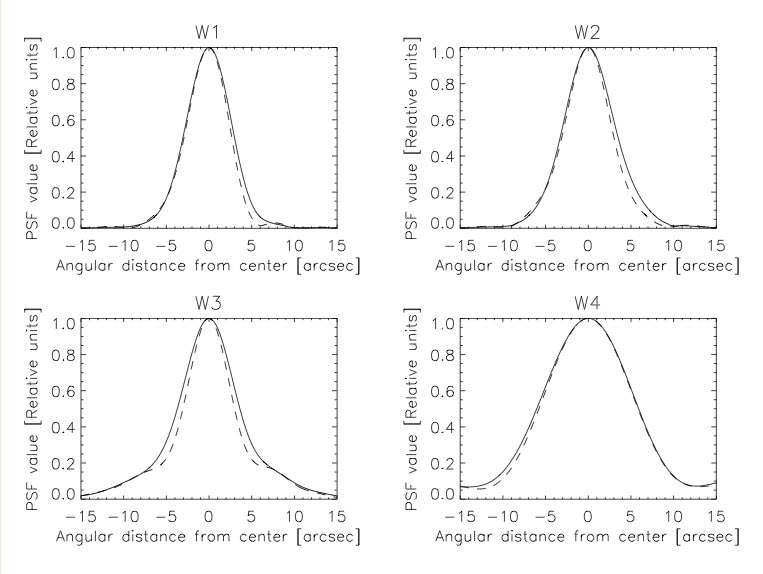
Profiles through the central PSF in the 9x9 array in each band are shown in Figure 8. The major axis has been defined as that for which the FWHM is maximized, and the minor axis is perpendicular to that.

Figure 8 - PSF profiles through major axes (solid lines) and minor axes (dashed lines).

The major and minor axes and position angles of major axes of the central PSFs are then as follows:

Noise pixel estimates can be found in IV.6.d.i.

2. WPRO Output Parameters

• ra, dec: right ascension & declination (degrees J2000)


• sigra, sigdec, sigraddec: position uncertainties of ra, dec and cross-terms, respectively (degrees J2000) (calculated using Equations 8 and 9)


• w?flux: integrated flux in DN units (This number can be negative)


• w?sigflux: uncertainty in the integrated flux in DN units (calculated using Equations 8 and 9)


• w?snr: signal-to-noise ratio (w?flux/w?sigflux). This value is NULL if w?flux is negative.


• w?mpro: integrated flux in mag units. If w?snr<2 this is the 2-σ magnitude upper limit (see below, IV.5.c.iii.3)


• w?sigmwpro: integrated flux uncertainty in mag units; this value is set to NULL if w?snr<2 (see below, IV.5.c.iii.3)


• w?rchi2: goodness of profile fit, reduced χ² for individual bands, as discussed in IV.5.c.iii, above.


• rchi2: reduced χ² for the composite four bands (Equation 7)


• nb: number of blend components including the parent (e.g., see Equation 3)


• na: number of active deblend components, determined using the active deblending procedure.


• w?sat: fraction of saturated pixels (see below, IV.5.c.iii.4). Note that pixels may be saturated for reasons other than source brightness; e.g. cosmic ray hits and "hot" pixels.


• w?frl: fraction of latent pixels (see below, IV.5.c.iii.4)


• SatNum: minimum sample (up the ramp) at which saturation occurs, whereby the saturation can be attributed specifically to high source flux. This is a string of 4 digits, one per band, with "0" representing non-saturation. Otherwise, the digit is in the range 2-9 for W1 and W2, and 1-9 for W3 and W4, with lower numbers representing more highly saturated cores of bright stars.

3. WPRO Magnitude Upper Limits

4. Saturation and Latent Fractions

w?sat: The number of saturated pixels located within the photometric "fitting" region in the vicinity of the source, expressed as a fraction of the total number of pixels within that region. The saturated pixels themselves were excluded from the solution, as explained above.

w?frl: The fractional number of pixels within the fitting region which were flagged as begin contaminated by latents. These pixels were also excluded from the solution.

5. Frame Detection and Flux Repeatability Statistics

1. N of M statistics

N of M refers to the number of S/N > 3-σ extractions relative to the total number of measurements for a source. Sources that are low S/N will have a low N/M fraction, and conversely high S/N sources should have a fraction that is unity. Those sources that are high S/N but exhibit a low N/M fraction may indicate measurement failures or source instability.



2. standard deviation of the population and the mean

The distribution in individual measurements has a mean and standard deviation of the mean and population. Sources that are high S/N but exhibit a large standard deviation may indicate short-time scale variability or measurement failure.

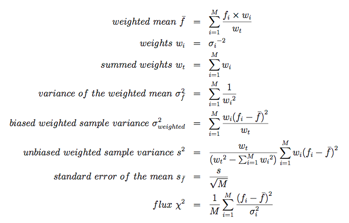(Eq. 23) (Eq. 24) (Eq. 25) (Eq. 26) (Eq. 27) (Eq. 28) (Eq. 29) (Eq. 30)

The weighted mean, the unbiased weighted sample variance (re: population variance) and the standard error of the mean are reported. Comparison of population variance with composite WPRO flux variance may be used to assess time variability; see next section.

Repeatability Output Parameters

• w?m: The number of individual frames that are available to make a profile-fit measurement.


• w?nm: The number of individual frames on which WPRO extracted a flux measurement that has SNR > 3.


• w?magP: mean (inverse variance-weighted) integrated flux in mag units (Equation 23)


• w?sigP1: unbiased weighted sample standard deviation (Equation 28)


• w?sigP2: standard error of the mean (Equation 29)

iv. System (WAPPco)

It should be understood that the profile fitting system (WPRO) represents the most accurate flux estimation for point sources under most circumstances -- the exceptions are when the source is high S/N (>> 50) but not saturated or when it is resolved and extended. Circular aperture photometry provides a better flux estimation for both of these cases.  If the source is associated with a 2MASS extended source, then WAPPco provides an elliptical aperture measurement designed to capture a larger fraction of the source flux as described below.

The basic flow of the WPHOT co-add photometry system WAPPco is illustrated in Figure 9. Fixed serves several purposes, including:

• source flux estimation in support of profile-fitting photometry,
• construction of curve-of-growth data for aperture corrections,
• more accurate flux determination for very bright sources,
• serve as a truth measurement to test the robustness of profile-fitting photometry, and
• accurate source flux determination for extended sources
in which the PSF does not accurately model the light distribution.

Figure 9 - system flowchart

The primary functions of WAPPco is to carry out circular and local background estimation. It performs the initial (preliminary) flux measurements for source characterization by WPRO, and applies a full suite of circular apertures on the co-added mosaics. The aperture MASK is scanned for bad, saturated or fatal-flagged pixels, and the aperture flux is flagged accordingly. If nearby stars are detected within the aperture, the flag is set to indicate "contamination." If the source is associated (in position) with a 2MASS XSC source, elliptical is carried out using an aperture based on the 2MASS extraction. Finally, if the source is suspected to be extended (e.g., poor χ² value ), then it is flagged as such.

1. Special Inputs

2. Circular Apertures

• Standard Aperture Radius: 8.25 arcsec (W1, W2, W3) and 16.50 arcsec (W4)


• Full set of Aperture Radii:



bands	1	2	3	4	5	6	7	8	units
W1, W2, W3	5.50	8.25	11.00	13.75	16.50	19.25	22.00	24.75	arcsec
W4	11.00	16.50	22.00	27.50	33.00	38.50	44.00	49.50	arcsec



• Standard annulus radii: 50 to 70 arcsec (W1, W2, W3, W4); see also IV.6c.ii.2.


• Aperture Correction: PSF-corrected_flux [mag] = measured_flux [mag] - aperture_correction:



W1	W2	W3	W4
[mag]	[mag]	[mag]	[mag]
0.222	0.280	0.665	0.616

Multiple is the primary function of the WAPPco system. The standard aperture is used to measure the source brightness in a small aperture, which is then corrected so that it recovers the "total" flux of the source, thus matching the PSF-measured flux of the source. A set of nested circular apertures centered on the source (as determined by WPRO) provides the "curve of growth" for a source. The aperture sizes range from the smallest APMIN (5.5 arcsec, or 4 co-added pixels) to the largest APMAX (24.75 arcsec, or 18 co-added pixels), which is constrained by the background annulus. The photometry is carried out using code, developed by 2MASS, that is adapted for WISE images. It includes fractional pixel computations and the ability to use non-circular (elliptical) apertures that are deployed for measurements of 2MASS XSC galaxies.

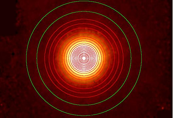Figure 10 - Set of nested circular apertures (red) and background annulus (green).

Formal aperture and error model measurements (see also II.3.f):

(Eq. 31) (Eq. 32) (Eq. 33) (Eq. 34) (Eq. 35)

where G is the gain (electrons per DN), N_ap is the number of pixels in the circular aperture of radius R_ap, N_b is the number of pixels in the background annulus, b_λ and σ_bann_λ are the sky background level and uncertainty in the annulus pixel distribution, respectively, σ_ann_λ is the uncertainty due to the finite annulus, and σ_b_λ is the measurement uncertainty detector/frame pixel based on the error model (see Eq. 1) and the estimated confusion noise, F_a and F_b are the pixel correlation factors, where they are roughly equal to each other. For WISE co-added images, the F values appropriate to the standard circular apertures (8.25 arcsec radius) are set to 32, 37, 58 and 221 respectively for W1, W2, W3 and W4.

3. Output

• w?mag: standard aperture-corrected magnitude (derived from Eq. 32); for low S/N measurements, an upper limit is used (see IV.5.c.iv.5)


• w?sigm: standard aperture-corrected magnitude uncertainty (derived from Eq. 35); for upper limits, the value is set to NULL (see IV.5.c.iv.5)


• w?flg : standard aperture confusion flag (see below)


• w?Cov: mean coverage depth within the circular aperture, whose float(real) value approximately corresponds to integer M (Eqs. 23-30)


• w?mag_n: circular aperture magnitude for aperture "n" (see above, for full set of apertures)


• w?sigm_n: circular aperture magnitude uncertainty for aperture "n"


• w?flg_n: circular aperture confusion flag (see below)


• w?Rsemi: semi-major axis (arcsec) for elliptical (IV.5.c.v below)


• w?ba: axis ratio (IV.5.c.v below)


• w?pa: position angle (E of N) (IV.5.c.v below)


• w?Gmag: elliptical aperture magnitude (IV.5.c.v below)


• w?Gerr: elliptical aperture magnitude uncertainty (IV.5.c.v below)


• w?Gflg: elliptical aperture confusion flag (see below)

4. Confusion and Warning Flags

flag values:

value    Condition
-----    ------------------------------------------------------
  0      nominal -- no contamination
  1      source confusion -- another source falls within the measurement aperture
  2      bad or fatal pixels:  presence of bad pixels in the measurement aperture (bit 2 or 18 set)
  4      non-zero bit flag tripped (other than 2 or 18)
  8      corruption -- all pixels are flagged as unusable, or the aperture flux is negative;
         in the former case, the aperture magnitude is NULL;  in the latter case, the aperture magnitude is a 95% confidence upper limit
 16      saturation -- here are one or more saturated pixels in the measurement aperture
 32      upper limit -- the magnitude is a 95% confidence upper limit

combinations:

  3      source confusion + bad pixels
  5      source confusion + non-zero bit flag
  6      bad pixels + non-zero bit flag
  7      source confusion + bad pixels + non-zero bit flag
  9      source confusion + corruption
 10      bad pixels + corruption
 11      source confusion + bad pixels + corruption
 12      non-zero bit flag + corruption
 13      source confusion +  non-zero bit flag + corruption 
 14      bad pixels +  non-zero bit flag + corruption
 15      source confusion + bad pixels +  non-zero bit flag + corruption
 17      source confusion + saturation
 18      bad pixels  + saturation
 19      source confusion + bad pixels  + saturation
 20      non-zero bit flag +  saturation
 21      source confusion + non-zero bit flag +  saturation
 22      bad pixels  + non-zero bit flag +  saturation
 23      source confusion + bad pixels  + non-zero bit flag +  saturation
 24      corruption + saturation
 25      source confusion + corruption + saturation
 26      bad pixels  +   corruption + saturation
 27      source confusion + bad pixels  +  corruption + saturation
 28      non-zero bit flag +  corruption + saturation
 29      source confusion + non-zero bit flag +  corruption + saturation
 30      bad pixels  + non-zero bit flag +  corruption + saturation
 31      source confusion + bad pixels  + non-zero bit flag +  corruption + saturation

5. Magnitude Upper Limits

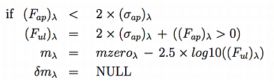
When the WPRO or WAPP flux measurement has a signal-to-noise ratio less than 2, the respective WPRO or WAPP calibrated magnitude in the Working Database is replaced with the 2-σ brightness upper limit in magnitude units. In these cases, the magnitude uncertainty values are set to NULL.

The magnitude upper limit is computed by replacing the integrated flux measurement with the flux measurement plus two times the measurement uncertainty, as shown below. If the integrated flux measurement is negative, then the flux is replaced with two times the flux uncertainty.

	(Eq. 36)
	(Eq. 37)
	(Eq. 38)
	(Eq. 39)

where mzero_λ is the instrumental zero point magnitude (IV.3.g.iv), m_λ is the reported upper limit in mag units, and its uncertainty δm_λ is set to NULL.

v. 2MASS Galaxies and Elliptical Apertures

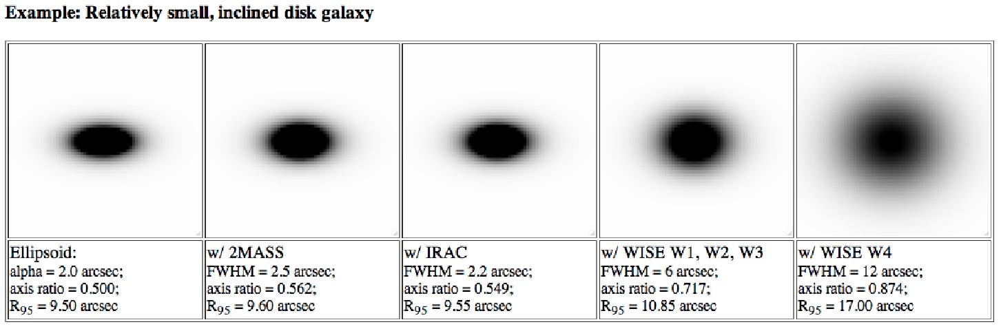
Sources that are in close proximity (xscprox <= 2 arcsec) to 2MASS XSC sources are assumed to be associated (i.e., the same source), and special is triggered for the source. The aperture is based on the elliptical shape that the 2MASS XSC reports. Due to the larger WISE beam, however, the aperture is adjusted (scaled) accordingly. Fig. 12 illustrates the difference in beam between 2MASS, IRAC and WISE, and the plots (Fig. 13-14) that follow show the quantitative difference which WAPPco uses to adjust the elliptical aperture for a particular case (XSC size and inclination). For a full suite of sizes and shapes, a lookup table is created to adjust the WISE aperture in accordance with the 2MASS XSC aperture shape.

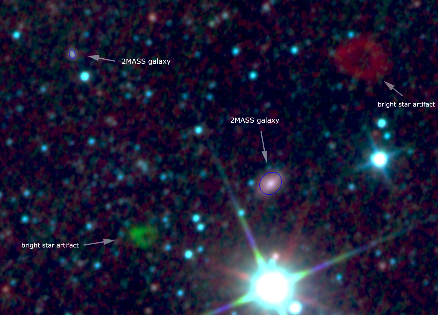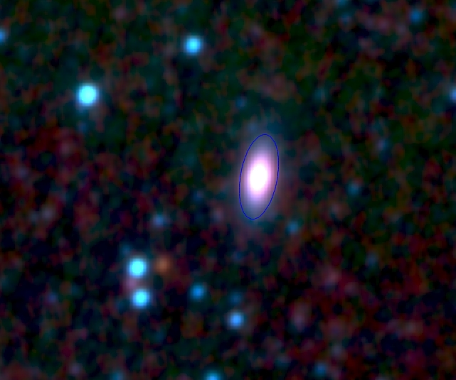
Figure 11 - WISE W1+W2+W3 composite image showing the elliptical aperture (blue) used to extract the flux from 2MASS galaxies in the field.

Figure 12 - Comparing 2MASS, IRAC and WISE beam-convolution of an ellipsoid model. the ellipsoid is defined as: f = f0 * exp(-r / alpha), where r is the radius based on the ellipse with axis ratio and position angle parameters; R95 represents the semi-major axis at which 95% of the total flux is captured.	Figure 13 - Semi-major axis of the disk galaxy compared to the actual radius due to the beam resolution.	Figure 14 - Axis ratio departure from 0.5 due to the beam resolution.

vi. Resolved Sources

There are two simple ways to assess whether a source is extended. Although they are not fool-proof, they are reliable, at least in the sense that they are a good warning signal. The two methods are WPRO rchi^2 thresholding and XSC proximity. For each band, the reduced chi^2 is a measure of the goodness of fit between the source and the PSF. The nominal value for this parameter is unity. For sources that are poorly fit, the value exceeds 2, and is often much larger. Resolved 2MASS galaxies exhibit large rchi^2 values, with typical values near 4 to 6 for the W1 measurements. Placing a threshold on the rchi^2, in any band, separates point-like from extended sources. This threshold should be some value between 2 and 4, where 2 is a stringent threshold and 4 is more relaxed.

• Define: w?rchi2 >= 3 in any band, then set the flag to extended

• Define: XSCprox <= 5 arcsec, then set the flag

Examples:

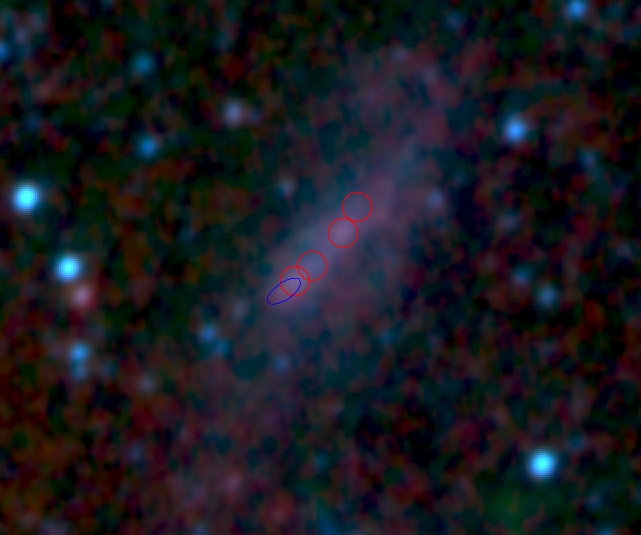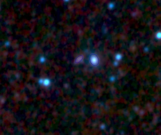
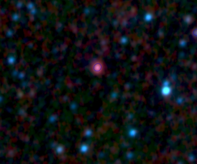
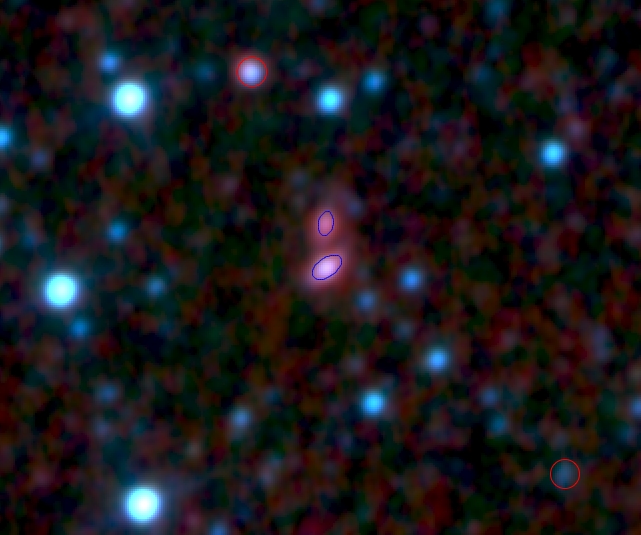
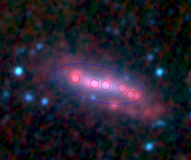
Figure 15 - Aperture (blue) used to extract W1 flux. The aperture is derived from 2MASS XSC.	Figure 16 - Two galaxies in close proximity, one is late-type star-forming and the other is early-type.	Figure 17 - Galaxy light arising from star-formation (W3 at 12-microns). The aperture (blue) appears to be too small, likely due to the K-band (2-micron) aperture model sensitive to old stars.	Figure 18 - Two star-forming galaxies, light arising from W3 (12-micron). The K-band aperture (blue) appears to be too small.	Figure 19 - Late-type galaxy with ill-defined nucleus. The 2MASS position is off-nucleus, peaking on a bright star-forming knot. Four WISE detections (red) along the disk have poor rchi^2 extractions.

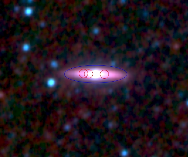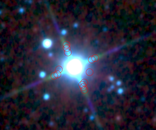
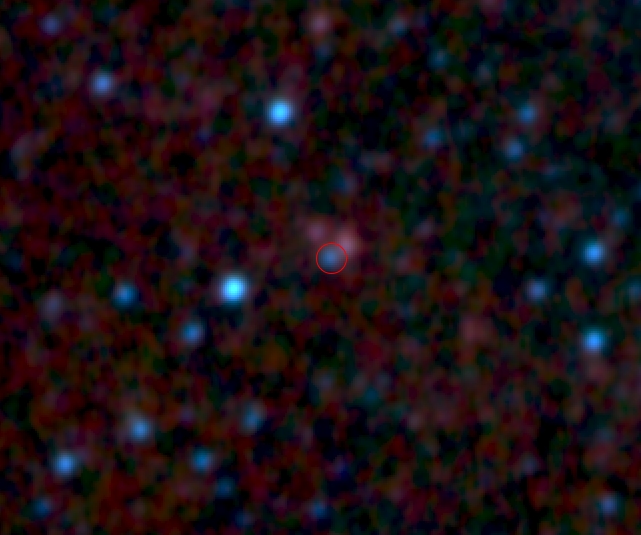
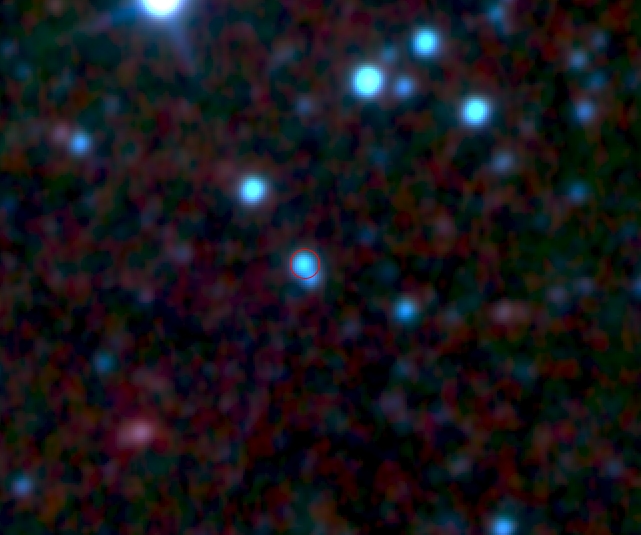
Figure 20 - Bright star artifact (diffraction spikes) inducing detections and subsequent poor photometric extractions (red circles).	Figure 21 - Star blended with two background galaxies.	Figure 22 - Star blended with another star.	Figure 23 - Late-type galaxy with weak nuclear emission. Pieces of the galaxy are detected and extracted (red circles) along the disk. One of the extractions, however, has a 2MASS XSC-derived aperture (blue) that is used to integrate the galaxy light.	Figure 24 - S0-type galaxy, with three point-source extractions (red; all have poor profile photometry). The galaxy aperture (blue) appears to be correct.

Last update: 2011 November 28