IV. WISE Data Processing
5. Multiframe Pipeline
c. WISE Photometry System (WPHOT)
iii. Profile-Fitting Photometry
4. Variability and Flagging
Overview
The variability flag, var_flg, is a four-character string with one character per band, consisting of integers that gives a measure of the probability that the catalog source is variable in each band. The flag is generated by analyzing single exposure measurements in the multiframe pipeline, but does not use the level 1b flux measurements. A value of "0" indicates insufficient or inadequate data to make a variability determination. Values of "1" through "9" indicate increasing probabilities of variability. Values of "1" through "4" can generally be regarded as non-variable sources in that band. Values of "5" through "7" can be regarded as potentially variable with small amplitudes. Objects with a value of "8" or "9" are most likely flux variables in the given band.
Method
The method relies on a generating a chi-square distribution using the standard deviation of the individual flux measurements of each source (w?sigp1). As a first pass, sources are pre-filtered to eliminate sources that have inadequate or insufficient data available to make a variability determination. The following are the pre-filters used and a brief purpose of each:
Table 1 - Pre-filters and their definitions
| w?nm / w?m > 0.8 |
Reliability of single-frame measurements. Tthis helps to ensure there is a detection of the source in the level 1b image. These parameters ensure at least 80% of the frames have a single-exposure detection at the location of the source in the multiframe image. However, this does not ensure there are also Level 1b flux detections for the source, as the Level 1b and the multiframe fluxes are measured at slightly different positions. |
| w?rchi2 < 5.0 | This reduces confusion issues by ignoring high chi square values. High chi square values normally indicate confusion or a extended source, both of which are not suitable for variability flagging. |
| cc_flags = 0 in at least one band | Artifacts, especially diffraction spike artifacts, can produce variability since the artifact location and intensity can vary between frames. Variability flagging is unreliable in the presence of artifacts and is avoided. |
| w?m > 10 | Small depth of coverage produces unreliable statistics since outliers have a larger effect on the overall variability. This filter helps to ensure the variability is significant. |
| Single-frame SNR proxy > 5.0 | This helps to ensure there is a single-frame detection--see description of the proxy below. |
| w?snr > 5 |
The coadd SNR must be significant, otherwise there will be no Level 1b detections. This filter ignores sources that are too faint to have any Level 1b detections. |
| na = 0 |
Eliminates sources with active deblending, which indicates one more more close neighbors that can produce false variability. |
| nb < 3 | This again avoids confusion, which can generate variability. Tests showed that some known variables were still detected with nb = 2, so the threshold was set at this value. For sources with nb > 2, flux variations are seen due to confusion. |
| w?sigmpro not null in at least one band | There must be a multi-frame detection of the source. |
| w?sigp1 not null in at least one band | There must be single-frame measurements for the source. |
To help ensure the variability flag is applied to actual Level 1b detections of the source, a single-frame SNR proxy was generated. The single-frame SNR cannot be estimated simply by using the value w?snr / &radic(w?m) as the multi-frame SNR estimation includes PSF error. To force this relationship to work, the SNR of both single and multi-frame measurements for approximately 100,000 random sources were compiled. A linear fit was applied to the function
| Y(w?mpro) = [&radic(w?m) * (w?snr1b / w?snrc )] |
(Eq. 1) |
where w?mpro is the coadd magnitude of the source for a given band, w?m is the number of images that went into the coadd, w?snr1b is the SNR of the Level 1b source, and w?snrc is the SNR of the coadd source. The result, is that [ Y(w?mpro) * w?snrc ] / &radic(w?m) gives a reasonable estimation of the single-frame SNR as a function of magnitude.
The standard deviation of the population, &sigma, is determined in each band by taking the 65th percentile of w?sigp1 in magnitude bins of 0.50. These distributions are saved as a look-up table as functions of M and magnitude. They are later interpolated upon retrieval. There is an effective faint-magnitude cutoff at 16.0, 14.75, 10.75, and 7.0 for bands 1,2,3, and 4, respectively. This is due to the lack of usable data at these fainter magnitudes to make the look-up table, as most of the multiframe sources at these fainter magnitudes do not have Level 1b detections. Sources fainter than these magnitudes will always receive a variability flag value of "0" in the appropriate band.
For each source passing the pre-filters, the significance of its w?sigp1 above the non-variable population is determined using the chi-square statistic, with the number of degrees of freedom N = M - 1:
| &chi2 = M*(w?sigp1)2 / &sigma2 |
(Eq. 2) |
where M is the depth of coverage and &sigma is taken from the look-up tables. The probability density function is
| PN(&chi2) = P0 * (&chi2)[(N / 2 - 1] * e-&chi2 / 2 |
(Eq. 3) |
where
| P0 = 1/[2N/2*&Gamma(N/2)] |
(Eq. 4) |
P0 normalizes the integral and &Gamma is the Gamma Function. Integrating PN from zero to the value of the chi-square statistic computed for the source and band, and subtracting from 1, gives the probability, Q, that the suspected variability (or one giving a statistic at least as large as that observed) occurred by chance. We then define F as the quantity that goes into the var_flg string for each band, as
| F = Floor[-log10(Q)] |
(Eq. 5) |
F is clipped at 9 for F > 9.
It should be noted that the var_flg values cannot be replicated using Level 1b flux measurements. The algorithm uses the standard deviation of the flux measurements from the single-exposure frames in the multiframe pipeline. These flux measurements are taken at the position of the catalog source, which can differ slightly from the location of the source in the Level 1b images. Therefore, the fluxes used in the calculation of w?sigp1 are not the same as the Level 1b flux measurements.
Results
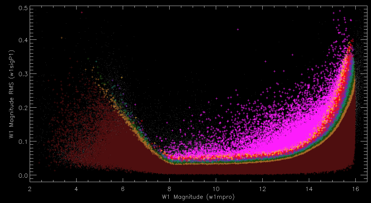
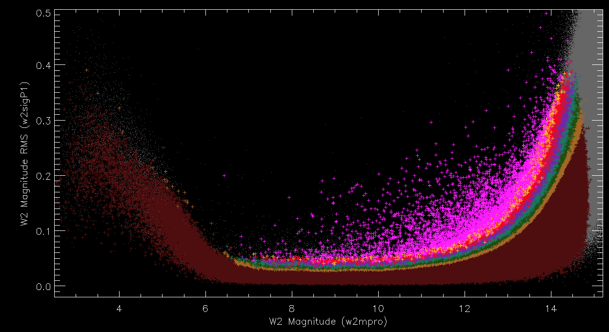
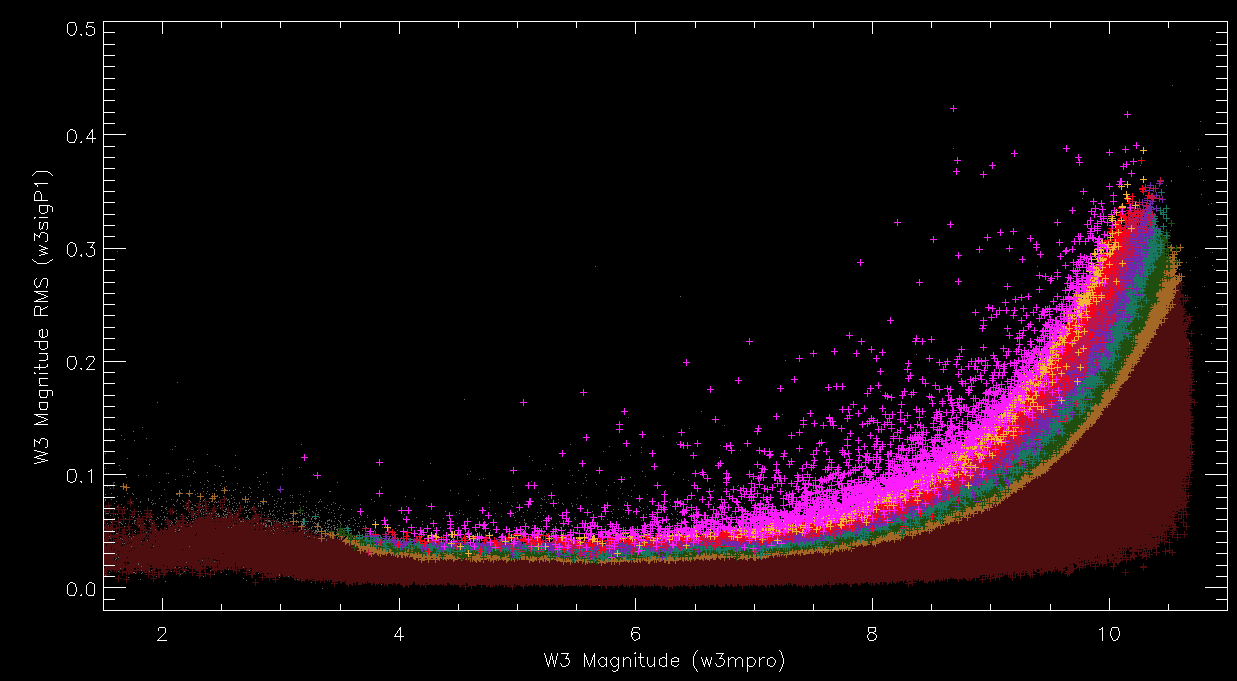
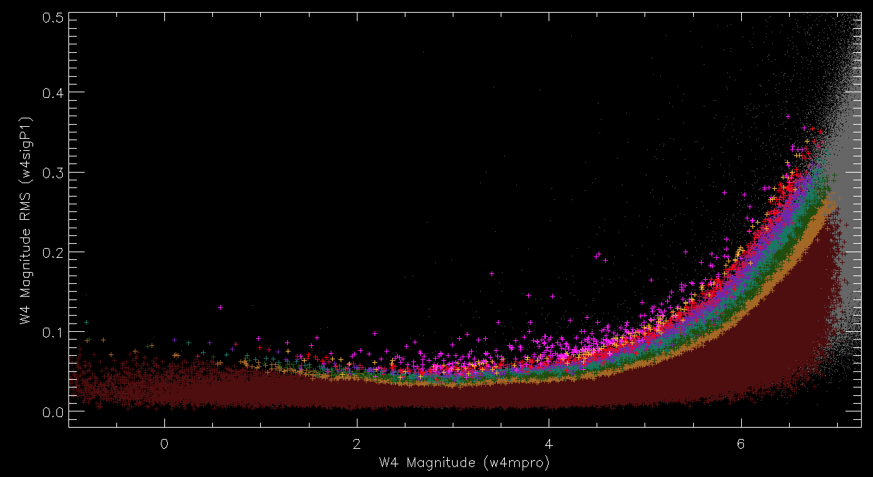
Figures 1-4 are graphical representations of the method applied to a large fraction of the sources in the preliminary data release. In each plot, the magnitude and w?sigp1 are plotted for sources. The small grey dots are catalog sources with F = 0, thus have inadequate or insufficient data to make a variability determination. F = 0 sources dominate the distribution, as M <= 10 coverage is very common, as are artifacts, and confusion. Sources flagged as artifacts and sources with low coverage are not plotted for clarity. The different colors represent different F values that are non-zero, ranging from F=0 (maroon) to F=9 (magenta). Known variables are generally safely in the F=9 region, with large amplitude variations. Sources with variability in W3 and W4 are quite rare due to the extensive artifacts and the smaller number of total sources in those bands.
 |
 |
| Figure 1 - Plot of a large subset of the preliminary release data in band 1. Grey dots are sources with F=0. Maroon crosses are the least variable sources (F=1). Different colors represent different F-values to to F=9 (magenta crosses). The white triangles in the W1 plot are sources with known and confirmed WISE variability. |
Figure 2 - Same as Figure 1 for band 2. |
 |
 |
| Figure 3 - Same as Figure 1 for band 3. |
Figure 4- Same as Figure 1 for band 4. |
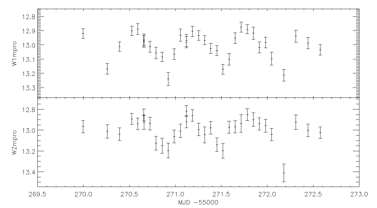
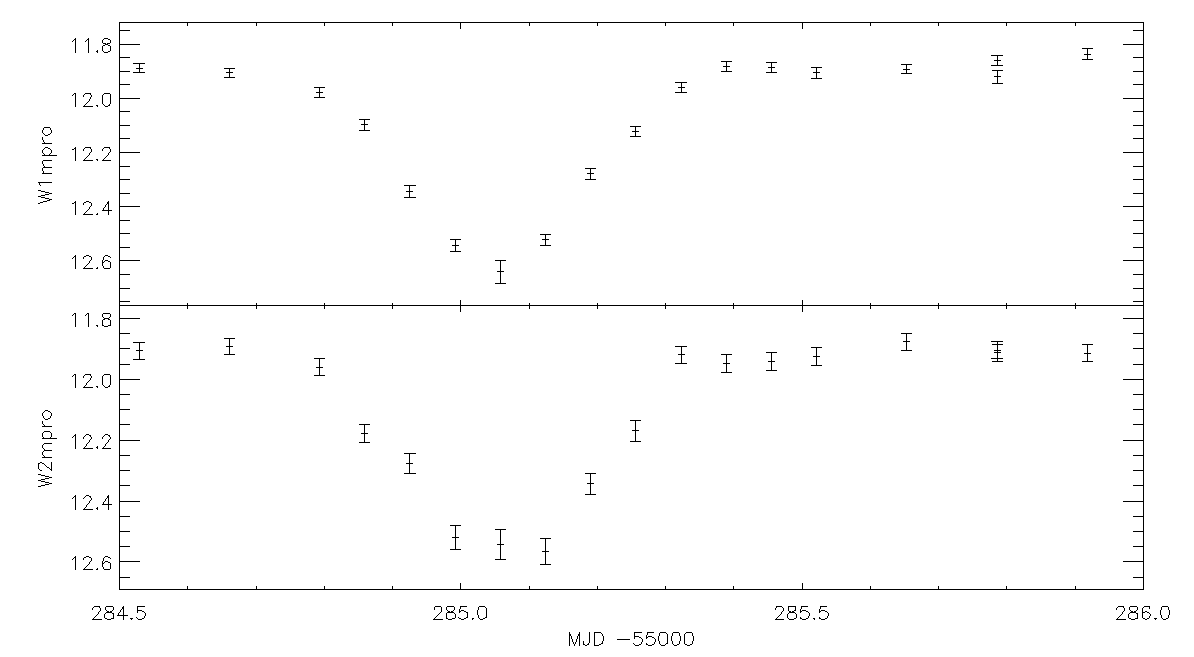
Figures 5 and 6 are two example light curves of sources with high variability values in both band 1 and 2.
 |
 |
| Figure 5 - An example RR Lyr light curve with a variability flag of '9900'. |
Figure 6 - An example Eclipsing binary light curve with primary eclipse with a variability flag of '9900'. |
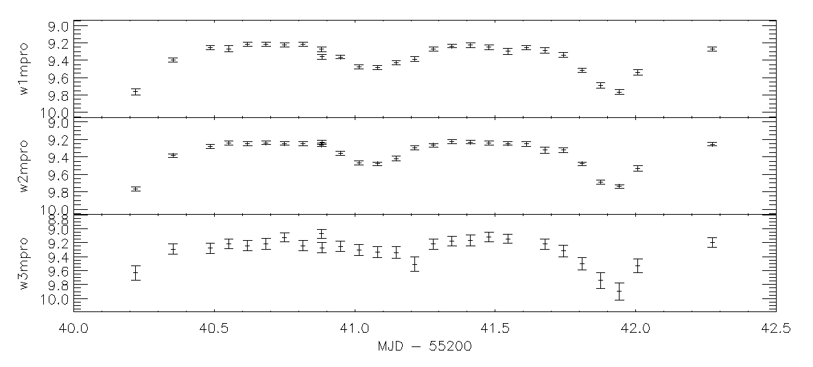
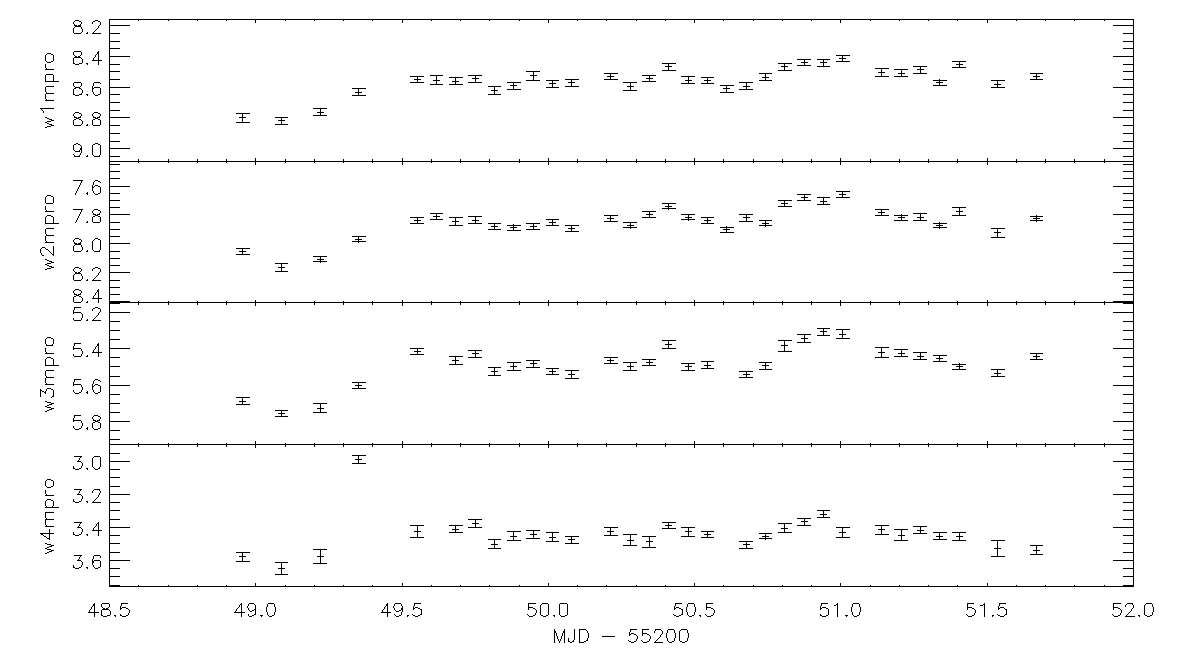
Figures 7 and 8 illustrate objects with variability in bands 3 and 4. In Figure 8, bands 1-3 are assigned F=0 due to the catalog source being flagged as an artifact in those bands. In this case, the artifacts do not appear to affect the light curve.
 |
 |
| Figure 7 - An example eclipsing binary light curve with primary and secondary eclipse. The variability flag is '9990' for this object. |
Figure 8 - An example of an object variable in all bands. The object is ET Cha, an Orion-type variable. The variability flag for the object is '0009'. The values are '0' for bands 1-3 because of artifact flags. |
Figure 9 is a light curve that illustrates a limitation of the algorithm. The source is an eclipsing binary, however, the var_flg string is '9100'. The source is bright enough in W1 where the short deviation of the eclipse is great enough to produce a significant RMS departure from the reference population. However, in band 2, F=1, and the source is classified as non-variable, even though the eclipse is obvious in the light curve. This happens because the reference RMS for the magnitude in W2 is higher than in W1, and the few deviant flux measurements near the eclipse are not enough to produce a significant RMS departure. This issue will be addressed in the final WISE release.
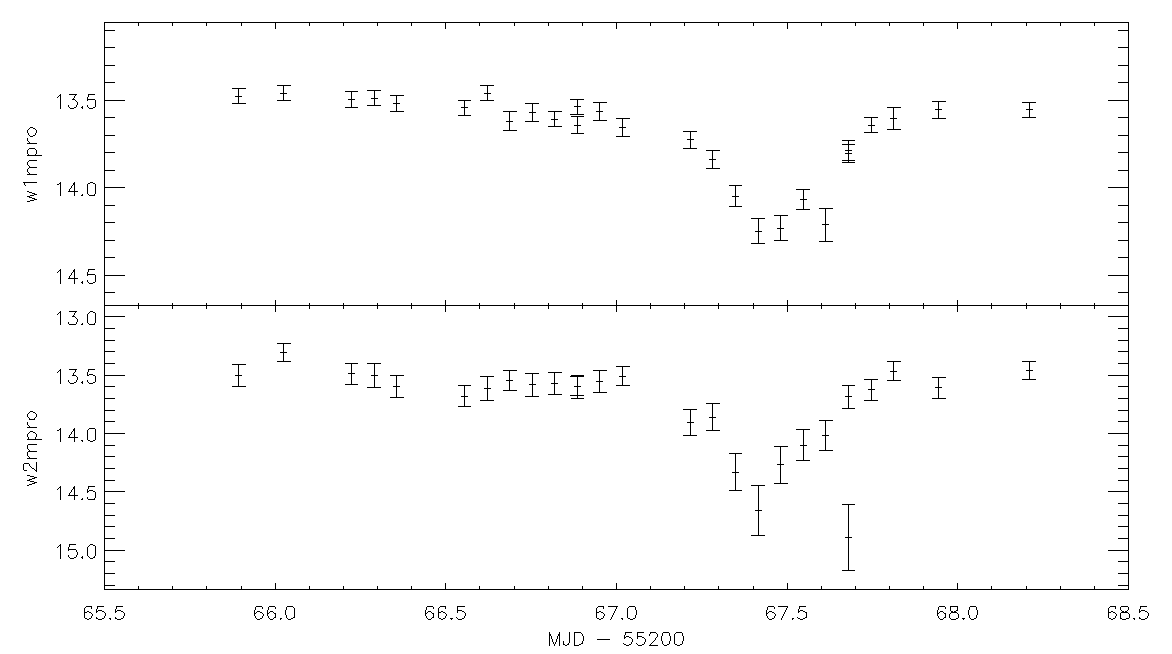 |
Figure 9 - An example of a problem where band 2 gets assigned F=1 despite an obvious eclipsing binary light curve. See text for details. |
Sources with F=8 or F=9 can generally be regarded as safely variable. Variability in sources with F=7 starts to become more uncertain. While the majority of F=7 are still variable, many of the known issues discussed in the next section start to become more common. Figure 10 illustrates a source that has a variability flag of '7100'. In this case, W1 is still statistically variable, although the amplitude is quite small compared to the error estimates. Band 2 in the same figure is non-variable and received a value of F=1.
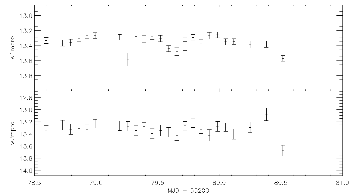 |
| Figure 10 - A source with a variability flag of '7100', illustrating marginal variability in W1 and no variability in W2. |
Known Issues
There are some known limitations with the variability flagging algorithm.
- Nebulosity around the source can create false variability. Because the multiframe and Level 1b source locations are slightly different, the multiframe measurement of the single-exposure frames is affected by slight variations in the nebulosity intensity as each frame probes slightly different locations.
- Unflagged artifacts (mostly from off-frame sources) contribute to variability.
- Flagging of artifacts is sometimes too aggressive, which leads to many F=0 variability flag values where light curves are generally unaffected.
- A close companion can increase the noise of the measurements, increasing the variability. This is reduced greatly by the na and nb constraints, but some still make it through.
- Non-rejected satellites/CR boost w?sigp1 with a single frame, leading to false variability (fairly rare).
- The population distribution of w?sigp1 does not follow a gaussian or chi-square distribution, but is close to a chi-square. The upper-percentile cut for σ is a correction.
- The method is not sensitive to short-lived, low-amplitude, transient events.
- Despite the largely successful attempt to estimate the single-frame SNR from the coadd SNR, magnitude, and number of frames, some sources are flagged as highly variable and have few, if any, level 1b detections in the given band.
Using the Variability Flag in Searches
When incorporating the variability flag into catalog searches, remember that the flag is a string. The user will likely need to make use of SQL code in searches. For example, to limit your search to sources with F>7 in W1 and W2 and F>5 in W3, the search string after the "where" clause would be:
var_flg[1]='[8-9]' and var_flg[2]='[8-9]' and var_flg[3]='[6-9]'
The search "var_flg matches '[8-9][8-9][6-9]?'" would also execute the same search in a more compact form. In most cases, it is best to place a constraint on at least two bands to lower the likelihood of one of the known issues driving the variability. When trying to exclude variability, remember that a value of "0" means insufficient or inadequate data to make a determination, and that "1" is the value to signify the least likelihood of variability in the band.
Last update: 2011 March 4
Previous page Next page
Return to Explanatory Supplement TOC