VI. Analysis of Release Products
2. Sky Coverage
In this section we describe the depth-of-coverage of the Preliminary Data
Release area and explain some of the issues with the pathologies of low coverage areas. For the
purposes of this section, the term "Sky Coverage" refers generically
to the topic of the WISE dataset spatial surveying features; when
appropriate, the term "depth-of-coverage" is used to refer
specifically to the number of observations at a specific point on the
celestial sphere, and the term "Catalog source density" is used to
refer to the number density of Catalog sources extracted in a small region.
The WISE survey strategy was designed to provide at least 8 frames
of coverage on at least 99% of the sky in the 6-month minimum all-sky
survey interval. This minimum coverage was required in order to
achieve sensitivity limits, and includes coverages lost due to
proximity to the Moon and the SAA, and further allows for recovery
period in the event of satellite anomaly (although no such anomalies
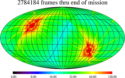
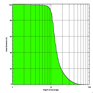
caused the loss of any data). As a result, the expected whole-mission
data downlink produce an ab initio depth-of-coverage as shown
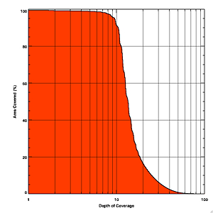
in Figure 1; the cryogenic portion of the
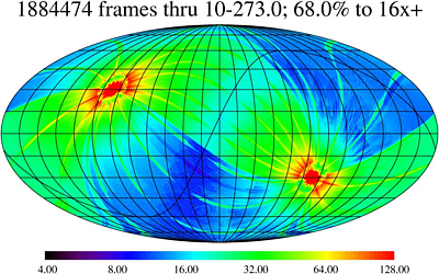
mission produces the coverage shown in Figure 2
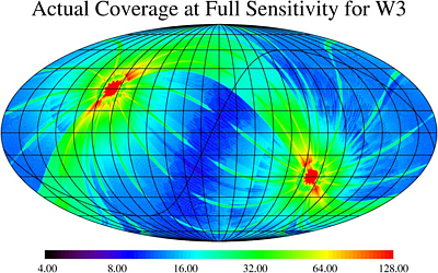
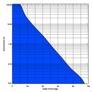
for bands W1 and W2. Because of the gradual degradation of performance
at cryogen loss, the depths-of-coverage of W3 and W4 vary slightly
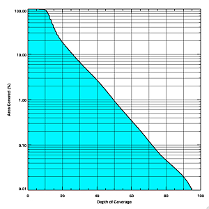
from that shown in Figure 2; these are shown
in Figure 3 and Figure
4.
 |
 |
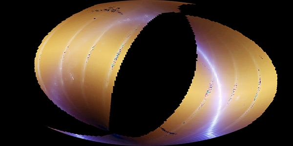
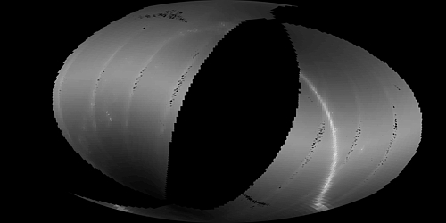
| Figure 1 - During the entire WISE operations period, covering more than a
year, a total of 2,784,184 framesets were taken and downloaded. The
depth of coverage across the whole sky in Galactic coordinates shows
the buildup near the ecliptic poles. |
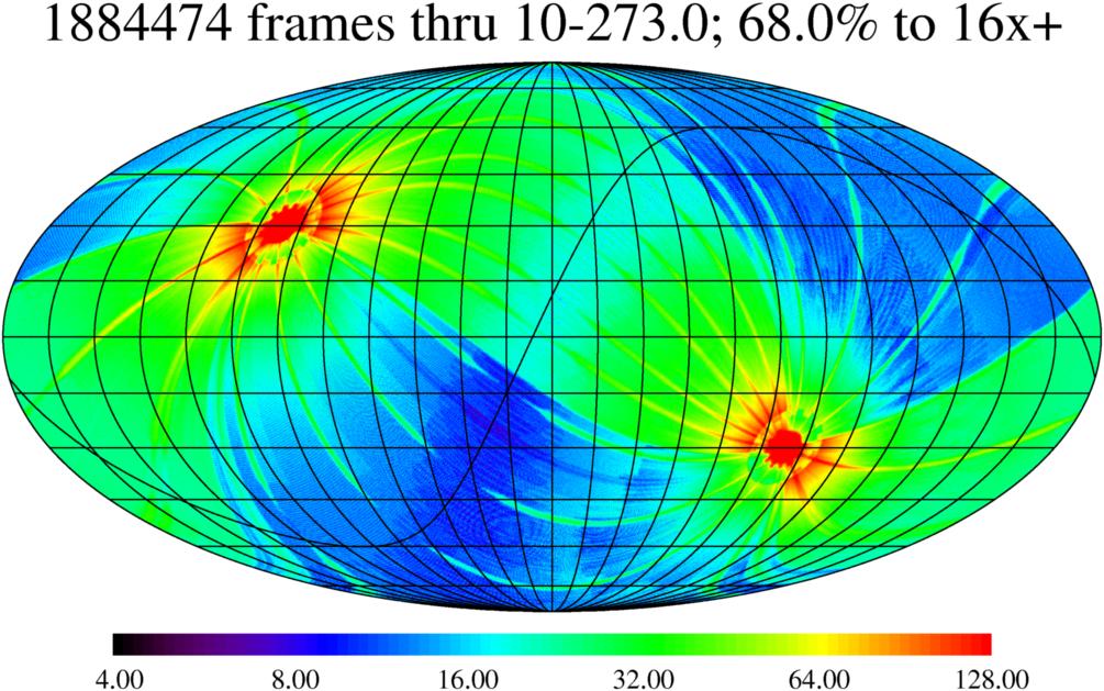
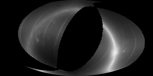
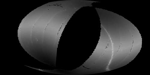
Figure 2 - The cryogenic portion of the mission, those framesets
which will be included in the Final Data Release, lasted until cryogen
depletion in October 2010. Up to that time, all W1 and W2 data cover
the sky at a depth of more than 8 using 18,844,474 framesets. |
 |
 |
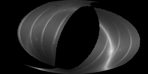
| Figure 3 - As WISE approached cryogen loss, the telescope began to
warm up. W3 integration times were reduced to prevent saturation once
the telescope had reached 45 K. The actual coverage at full
integration time is somewhat shallower for W1 and W2. |
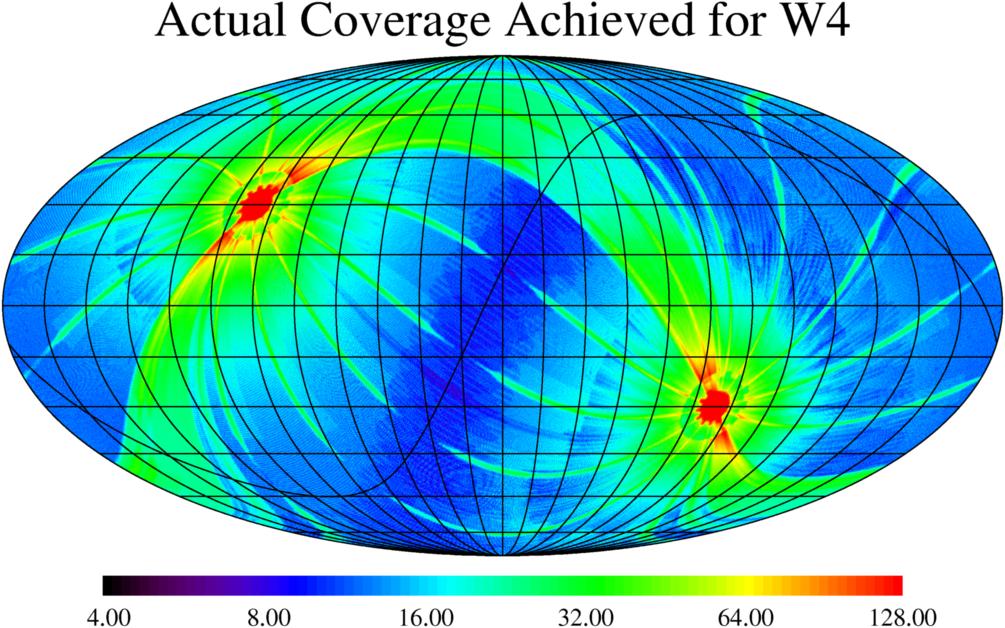
Figure 4 - As WISE approached cryogen loss, the telescope began to
warm up and the W4 detectors saturated. The actual coverage at 22
microns is therefore shallowest of all the WISE bands. Even so, the
nominal survey coverage allowed 99.92% of the sky to be seen 8 times
or more. |
a. Preliminary Data Release Area
The Atlas and Source Catalog of the WISE Preliminary Data Release
are drawn from data taken during the first 105 days of WISE survey
observations, as described in V.2.
Because of WISE's survey strategy, this region is oriented in ecliptic
coordinates and covers great circles in the ranges of:
28.7°<λ<133.4°
and 201.9°<λ<309.6°.
This totals
approximately 23,658 deg2, or 57.35% of the sky.
On online tool is available to determine if a particular location or
object is in the Preliminary Data Release area, and if so, provides
the address of the Tile in which it is located.
 WISE Preliminary Data Release Tile Lookup Service
The WISE Preliminary Data Release area is comprised of
10,464 Atlas Tiles, each Tile spanning 1.564° × 1.564° in 4095 × 4095 pixels at a resolution of 1.375′′ per pixel. These Tiles are delivered in FITS format image sets, consisting of an intensity image, the corresponding uncertainty image, and a depth-of-coverage map at each of the four WISE bands. The full sky is tessellated with a grid of 18,240 such Tiles on an equatorial projection for the purpose of combining the WISE single-exposure images and extracting final source information. The Tiles are distributed in 119 iso-declination bands with 238 Tiles on the celestial equator decreasing to six Tiles in the |δ|=89.35° declination band. Tiles are designed to overlap by 180′′ in RA and Dec on the equator, increasing in RA overlap towards the equatorial poles.
The ecliptic longitude boundaries of the Atlas and Catalog are pulled in from the original boundaries because of minimum coverage requirements.
The Release does not cover the ecliptic poles because those Tiles are not fully contained in the survey boundaries from the first 105 days.
The actual boundaries of the Atlas coverage area are not smooth in ecliptic longitude because the Atlas Tiles are laid out in an equatorial grid.
 |
|
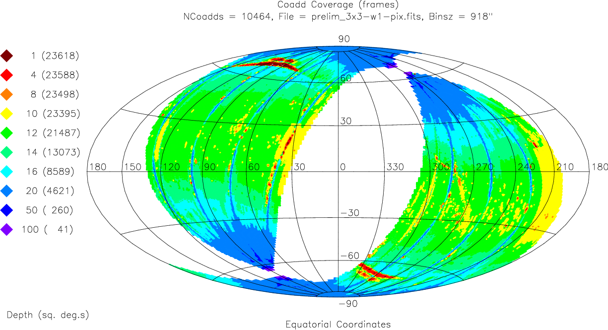
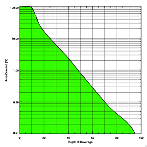
| Figure 5 - Equatorial aitoff projection sky map
showing the area covered by the WISE Preliminary Data Release. The
colors encode the average number of single 7.7/8.8 sec WISE exposure
frames covering 15´ × 15´ bins. The legend on the
left gives the cumulative area in square degrees as a function of
frame coverage depth. (Galactic and Ecliptic projections are
available in I.4.a.ii).
|
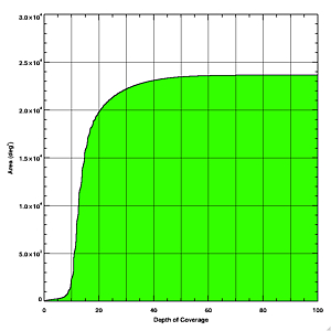
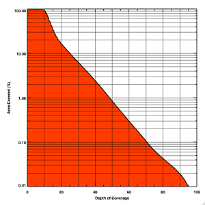
Figure 6 - Differential area as a function of average frame
depth-of-coverage in the Preliminary Release, computed in 15´
× 15´ bins. |
Below is a full-sky Aitoff equa-area projection of the WISE
Preliminary Data Release Atlas Images in equatorial coordinates. The slight
differences in coverage at the four wavelengths can be seen, as can
the strips of enhanced background due to the proximity of the Moon
(seen as segments running slightly clockwise of vertical). The plane
of the galaxy runs prominently throughout, as does a diffuse zodiacal
light component.
 |
| Figure 7 - Aitoff equal-area projection of the WISE
Preliminary Data Release intensity images, covering
23,658°2.
|
 |
 |
| W1 | W2 |
 |
 |
| W4 | W4 |
| Figure 8 - Aitoff equal-area projection of the WISE
Preliminary Data Release intensity images in each band.
|
b. Sky Coverage Statistics
WISE survey depth-of-coverage varies across the sky because of the survey
scanning strategy, as described in III.4.
There are typically 12 independent exposure frames contributing to each
point on the sky near the ecliptic plane. The depth increases towards the
ecliptic poles, reaching a maximum of ~260 frames at the highest
ecliptic latitudes in the Preliminary Data Release (Figure 5). Visible
in Figure 5 are some small patches with decreases in frame coverage
caused by filtering out exposures considered to be
of lower quality because of contamination by scattered moonlight
(within 20° of the ecliptic), image quality degradation due to
flight system motion, or other events. Pixel-level frame coverage
information is provided in the WISE Image Atlas
Depth-of-Coverage Maps. Here we present ensemble statistics of the
coverage achieved for this data release.
Each Atlas FITS image contains in the header
some high-level quantification of the depth-of-coverage for that Tile.
This information may also be accessed in the Atlas
Inventory metadata table. (Full depth-of-coverage information can
readily be derived from the Atlas Depth-of-Coverage
maps, for those who
wish to determine this on a per-pixel level). The header keywords are
listed in Table 1.
Table 1 - Atlas Image FITS Keywords Describing Depth-of-Coverage
| Keyword | Meaning | Data Type |
| MEDCOV | Median depth-of-coverage | float |
| MINCOV | Minimum depth-of-coverage | float |
| MAXCOV | Maximum depth-of-coverage | float |
| LOWCOVPC | Percent of pixels with depth ≤5† | float |
| NOMCOVPC | Percent of pixels with depth ≤8‡ | float |
Notes:
† Coverage ≤5 implies pixels that are at or below the
threshold for statistically viable outlier detection and rejection
(see below), and so can be contaminated by random
pixel variations.
‡ Coverage ≤8 implies regions where the coverage is less
than the nominal coverage required for the stated minimum sensitivity
goals.
The median depth-of-coverage across the full Preliminary Data
Release Area is 13.79 in W1, 13.78 in W2, 13.26 in W3, and 13.55 in
W4. Below, we show more complete statistics of the depth-of-coverage
distributions in this data release.
 |
 |
| W1 | W2 |
 |
 |
| W3 | W4 |
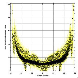
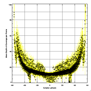
| Figure 9 - Calculated
depth-of-coverage vs. ecliptic latitude for each band; the yellow
region indicates the dispersion of the distribution in each Tile.
|
 |
 |
| W1 | W2 |
 |
 |
| W3 | W4 |
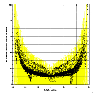
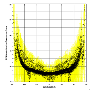
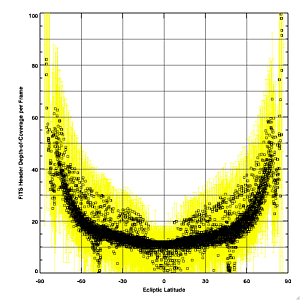
| Figure 10 - FITS header values of the
median coverage in each band vs. ecliptic latitude; the yellow region
indicates the minimum and maximum coverage in each Tile.
|
 |
 |
| W1 | W2 |
 |
 |
| W3 | W4 |
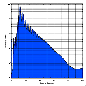
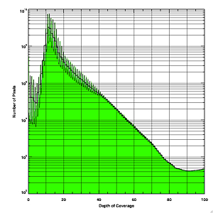
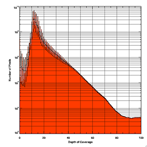
| Figure 11 - Histogram of per-pixel
depth-of-coverage in each Tile for each band for the entire
Preliminary Data Release. Note that this is summed over Tiles, and so
there is a slight overlap resulting in a double-counting of certain
spatial pixels on the sky.
|
 |
 |
| W1 | W2 |
 |
 |
| W3 | W4 |
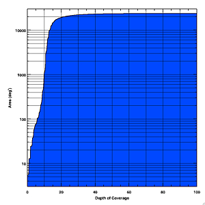
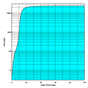
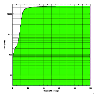
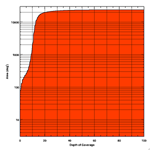
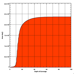
| Figure 12 - Cumulative histogram of
the area in square degrees resulting from integrating the curves
in Figure 11, above.
|
 |
 |
| W1 | W2 |
 |
 |
| W3 | W4 |
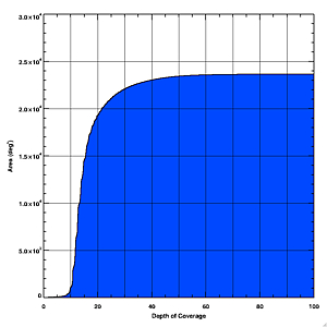
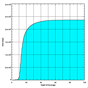
| Figure 13 - Same as Figure 12, but in a linear scale.
|
 |
 |
| W1 | W2 |
 |
 |
| W3 | W4 |
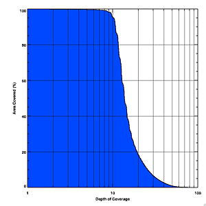
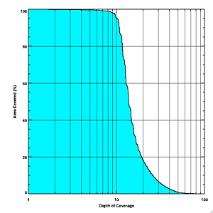
| Figure 14 - The ordinate shows the
percentage of the sky covered in the Preliminary Data Release Tiles to
a depth of at least that indicated on the abscissa, for each band.
|
 |
 |
| W1 | W2 |
 |
 |
| W3 | W4 |
| Figure 15 - Same as Figure 13, but in log-log scale.
|
c. Caveats About Low Coverage
The WISE scan strategy was designed to allow for repeat viewings of
at least 8 times on every point on the sky, with accommodations
allotted for planned survey motions and margins for unplanned survey
interruptions. The achieved characteristic coverage is slightly higher than
this because the survey was not interrupted. However, there are some
regions that have anomalously low effective coverage in the
Atlas Images and Source Catalog because some Single-exposure
framesets were rejected from Multiframe processing due to poor assessed
quality (i.e. see V.2).
Some of the reasons for low coverage are summarized below.
i. Torque Rod Gashes
Comparison of the achieved Atlas tile coverage (Figures 5, 7, and 8) with the survey frame coverage (Figures 1-4, also via interactive comparison) illustrates several areas with a notable loss of coverage within the general boundaries of the release. Most significant are the horizontal bands at Ecliptic λ,β= 100°,+45° and 290°,-45° (Equatorial α,δ= 110°,+70° and 310°,-70°).
Early in the survey, the spacecrafts' magnetic torque rods were enabled to dump accumulated momentum when scans approached within 45° of the ecliptic poles. Activating the torque rods resulted in a small jump in the telescope pointing and smearing of the resulting images.
Because the smearing occurred near the same point on each orbit, and the smeared images were flagged as having degraded image quality in the QA process, low-coverage "holes" developed at those locations. Later in the survey (2010 May 02), torque rod enabling was staggered between 45, 57.5 and 70° latitude on alternating orbits so that any image smearing would not occur at the same point on the sky on each orbit.
ii. Moon Contamination
When WISE observes near the moon, stray light can contaminate images
significantly enough that source detection sensitivity is degraded
and spurious detections are triggered by the structured scatter light.
Moreover, spatially-varying scattered light artifacts are problematic
for the background-matching portion of
the Multiframe pipeline image coaddition process.
The Moon crosses the scan circle twice a month. This would imply
that a large amount of data would be corrupted; this would leave gaps
in the sky coverage. To counter this, the WISE survey strategy
uses a modified scan pattern
where the scan circle gets slightly ahead before the Moon interferes and
then drops slightly behind to recover the region the Moon obscured.
The Moon moves 13° per day in ecliptic longitude, so with a 15° nominal
exclusion zone (30° diameter) WISE needs to be 1.2° ahead just
before the Moon crosses the scan circle, and then drops back to
1.2° behind just after the Moon crosses the scan circle. This "Moon
avoidance" maneuver produces the "spokes" of enhanced coverage that are
visible in the nominal sky coverage maps seen in Figures 1-4, for example.
Moon avoidance helps to fill in the coverage, but does not solve the
problem fully because scattered light artifacts affected frames taken
as far as ~30° away in W3 and W4, and ~20° in W1 and W2.
(e.g. see II.4.a.ii).
To minimize the impact of scattered moonlight in Single-exposure images on
the coadded Atlas Images, frames suspected to be contaminated
are flagged if they fall within the area of a
static "moon-mask", and filtered out
from the coadding if the spatially-varying portion of the moonlight
produces a pixel RMS in excess of a threshold defined by frames not
within the static moon-mask area, as described in IV.5.a.vi.
There are a few cases where most or even all of the available
input frames touching parts of an Atlas Tile are within the masked region
resulting in incomplete rejection of the scattered light artifacts,
or, in the worst cases, zero-coverage holes in the Atlas Images and
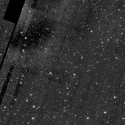
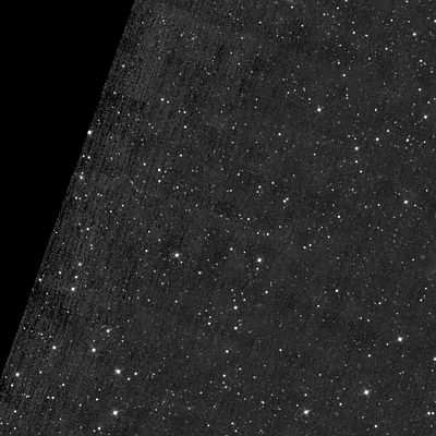
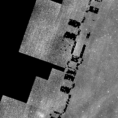
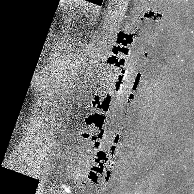
Catalog. An example of such an Atlas Image, 0333p181_aa11, is shown in
Figures 16 and 17. Because the extent of scattered moonlight is larger
in W3 and W4, the loss of coverage is more severe in those bands.
 |
 |
| W1 | W2 |
 |
 |
| W3 | W4 |
| Figure 16 - Atlas Intensity Images for Tile 0333p181_aa11,
showing residual scattered light and loss of coverage because of Moon
contamination. The extent of scattered moonlight is larger at
longer wavelengths, so the resulting loss of coverage is greater. |
 |
 |
| W1 | W2 |
 |
 |
| W3 | W4 |
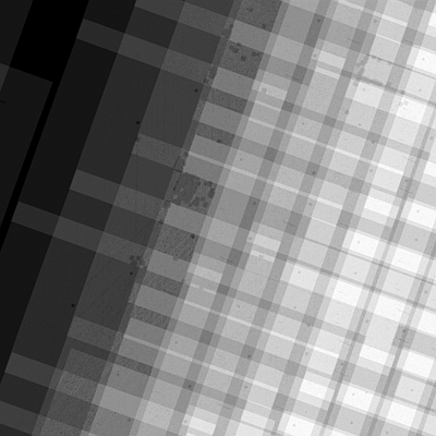
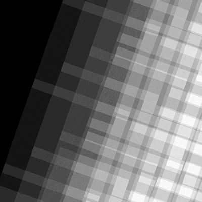
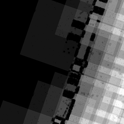
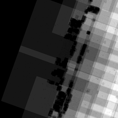
| Figure 17 - Corresponding depth-of-coverage map
for Atlas Image 0333p181_aa11 showing obvious Moon
contamination; the depth-of-coverage ranges from zero near the upper
left to ~12 towards the lower right. |
To assist in the proper identification of moon-contaminated Tiles,
there are FITS keywords in the Atlas Image headers
that describe the Moon contamination mitigation process. These are detailed
in Table 2. These parameters are also available in the
Atlas Inventory metadata tables. As an example,
for Tile 0333p181_aa11 in W1, the value of MOONINP
indicates that 47 frames (out of NUMFRMS=64 initial frames)
are flagged as "suspect" for moon-glow; of these, MOONREJ=45
were rejected, leaving only 19 frames to make up the final Tile. With
such extreme ratios, care should be taken with the portions of the
Tile nearest to the uncovered area. The WISE outlier detection relies
on median absolute deviation as a robust measure of the dispersion of
the pixel intensity distributions at any particular location. This
technique becomes unreliable below a depth-of-coverage of five, so
outliers may be incorrectly flagged and removed.
Table 2 - Atlas Image FITS Keywords Describing Moon Contamination
| Keyword | Meaning | Data Type |
| MOONREJ | Number of frames rejected due to moon-glow | int |
| MOONINP | Initial number of frames with suspect moon-glow | int |
| NUMFRMS | Final number of frames touching footprint | int |
iii. Source Density Suppression Around Bright Stars
Bright stars have a noticeable impact on depth-of-coverage, but
also a more subtle change in sky coverage as measured by the Catalog.
Very bright stars effectively obscure background sources with their
their scattered light halos and diffractions spikes, and they
elevate the surrounding background, thus increasing the
source detection limits.
This can be illustrated visually in an extreme case
for a very bright star, Betelgeuse. As a roughly -4th mag star,
Betelgeuse saturates thoroughly in each of the WISE bands, making it
an easy example for the effect. A by-eye inspection reveals the
suppression of source density in the vicinity of bright stars down to
a magnitude of ~5, and it is likely that this effect would be
statistically significant down to fainter levels.
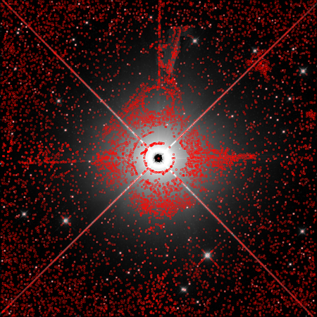
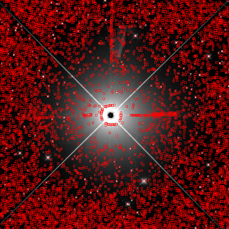
We show in Figure 18 the intensity in W1 for
a 54′×54′ region around Betelgeuse from Tile
0884p075. Overlaid on this are all the Catalog sources, including
those flagged as being contaminated by diffraction
spike objects, halo objects, etc. It is clear that the the distribution of
sources is spatially
nonuniform. One can infer that the source distribution is the result
of a high density of potentially spurious sources within the halo
area, a suppression of real sources in the halo near the bright star,
and the more-or-less-uniformly distributed real sources at a greater
distance from the star. The suppression of Catalog source density is a
subtle effect of bright stars that can lead to, for example, incorrect
two-point correlation function determination due to an unknown
windowing. This lack of sky coverage is not reflected in the
depth-of-coverage information provided in the Atlas Image sets.
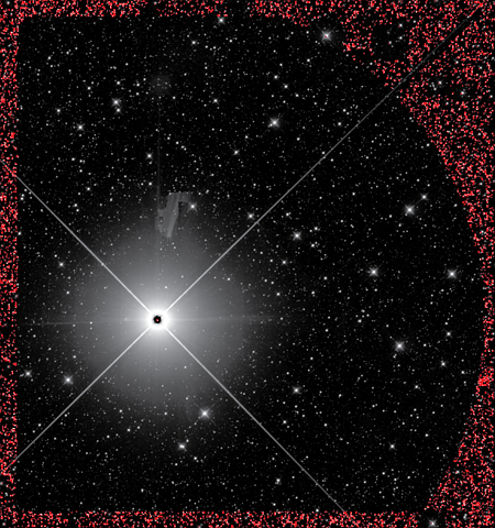
The example in Figure 18 shows the distribution of all Catalog sources,
but many of them are flagged to enable Catalog-query-based removal
of potentially contaminated sources. If one removes these
potentially contaminated and spurious sources by selecting only those
with cc_flags="0000," the
entire region is denuded of
sources, as shown in Figure 19.
 |
 |
| Figure 18 - Atlas Intensity Image in W1 for a
54′×54′ region around Betelgeuse from Tile
0884p075_aa11. Overlaid on this are all the Catalog sources, including
those flagged as diffraction spike objects, halo objects, etc.
|
Figure 19 - Intensity in W1 for a
54′×54′ region around Betelgeuse from Tile
0884p075_aa11. Overlaid on this are only the fully reliable Catalog sources
where cc_flags="0000."
A ~1.5° region near Betelgeuse is effectively blanked out.
|
Refined selection criteria can be used to eliminate
the spurious sources without filtering our all real objects. One way is
to also use the multiple-band detection bit flag,
det_bit,
since spurious sources should not necessarily be associated with the same
Catalog entry. Taking the above field and selecting according to:
(det_bit=3 or
det_bit=7 or
det_bit=11 or
det_bit=15) and
w1cc_map_str not like "d%" and
w1cc_map_str not like "D%"
results in an improved
likelihood of the reliability of sources (Figure 20), which makes it
more evident that the Catalog source density is low in the region of
bright stars.
 |
| Figure 20 - Intensity in W1 for a
54′×54′ region around Betelgeuse from Tile
0884p075. Overlaid on this are selected Catalog sources chosen to be detected in W1 and W2, removing many spurious sources and highlighting the Catalog source density suppression near Betelgeuse and other bright stars.
|
As one final note, we mention that the depth-of-coverage is low in the
immediate vicinity of bright stars. This is reflected in
the Atlas Image Depth-of-Coverage Maps files and
is visible in the depth-of-coverage
histograms as the regions of anomalously low coverage. It should be
noted there are also low depth-of-coverage groups of pixels
associated with the ghosts and latents of bright stars, as is shown
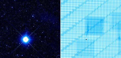
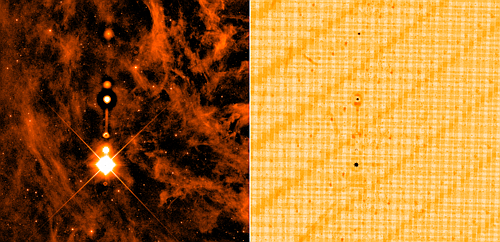
for W2, W3, and W4 in Figure 21. This shows
the intensity and coverage images near Betelgeuse for bands W2 (top), W3
(middle), and W4 (bottom). The ~zero depth-of-coverage right at the
position of the star is evident in all bands, as are the ~zero
depth-of-coverage latent
images in W3 and W4 that extend for several degrees.
 |
 |
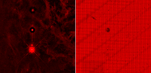 |
| Figure 21 - Intensity (left) and depth-of-coverage (right)
images near Betelgeuse for bands W2 (top), W3 (middle), and W4 (bottom).
The ~zero
depth-of-coverage right at the position of the star is evident in all
bands, as are the ~zero depth-of-coverage latent images in W3 and W4
that extend for several degrees.
|
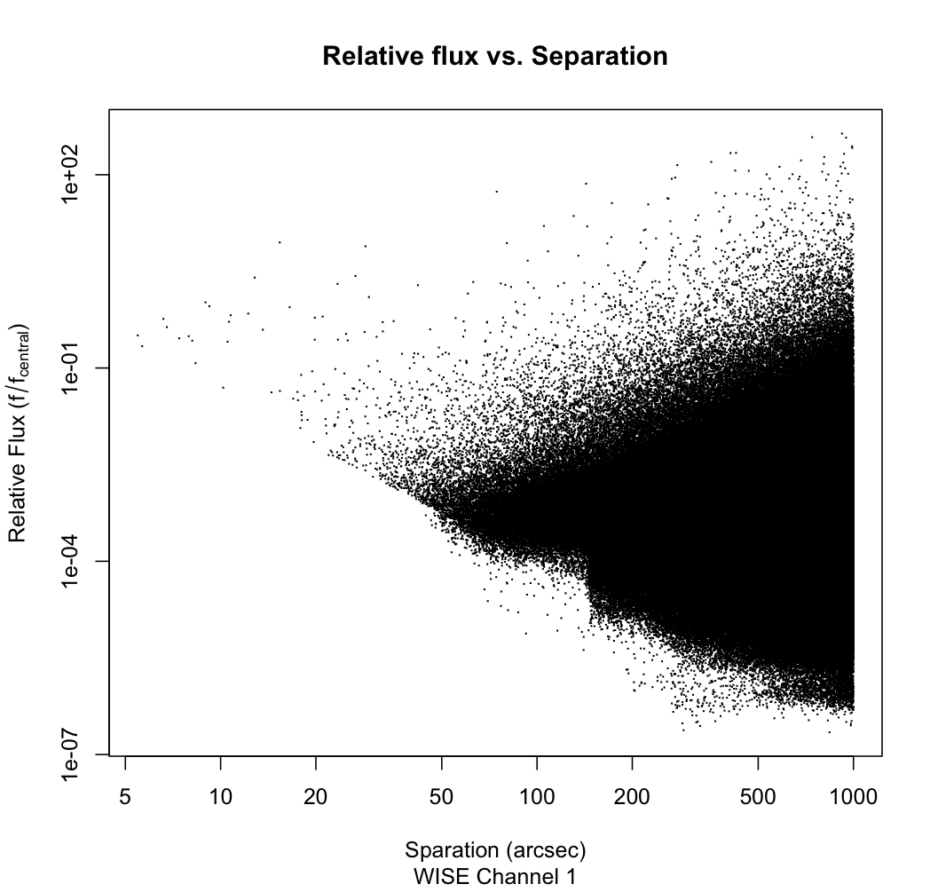
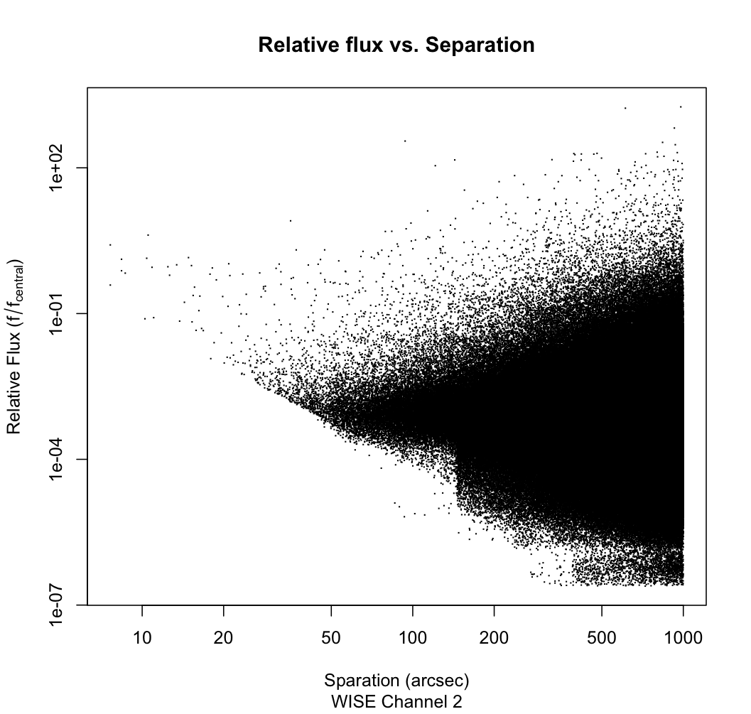
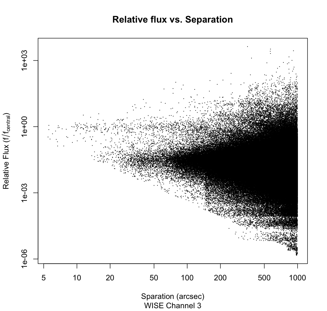
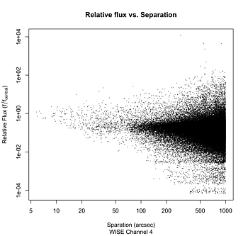
A quantitative analysis of the Catalog source density suppression has
been done for a large set of randomly-selected stars brighter than 9th
magnitude. As the plots in Figure 22 show, there is a lack of sources
near the bright star that suppresses other sources as a function of
radius, with fainter stars suppressed to greater radii.
 |
 |
| W1 | W2 |
 |
 |
| W3 | W4 |
| Figure 22 - Flux vs. separation
|
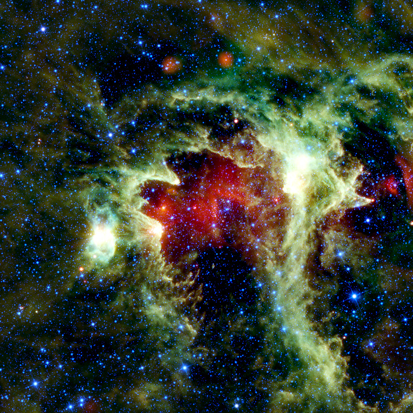
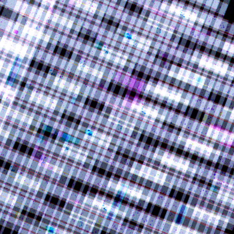
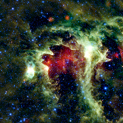
iv. High Flux/Source Density Regions
In regions with a large number of sources or particularly bright
sources (either diffuse or point-like), the depth-of-coverage can vary
between wavelengths in a spatially-varying way dependent on the
intensity structure. Hence, performing tasks such as aperture
photometry on extended sources must take into account these variations
across the source. As an example of the coverage variations, the
four-color composite intensity and depth-of-coverage maps for Tile
0450p605_aa11 are shown in Figure 23.
There is a pronounced decrease in coverage (in magenta color)
across a several arcminute-wide region just north of center and in the southeast in W3,
but not in the other bands. Similarly, some regions to the east of
center exhibit low coverage in W4 (cyan). These decreases are not
severe; the total stretch depth-of-coverage is roughly 12 to 19, while
the low coverage areas in those bands amount to a change in depth of
only a few. What is interesting about the spatial variations is that
the low depth-of-coverage is not coincident with the brightest regions
in the relevant bands, nor in the region of highest flux density. Such
decreased depths-of-coverage are to be anticipated and do feature in
this Tile.
 |
 |
| Intensity Image | Depth-of-Coverage Map (stretched) |
| Figure 23 - Four-color composite intensity and depth-of-coverage
images for Atlas Tile 0450p605_aa11, showing the reduced coverage in regions
with high background and around bright stars. Also note the pair of W4 latent
images near the top center of the image. |
Last update: 2011 April 26
Previous page Next page
Return to Explanatory Supplement TOC