IV. WISE Data Processing
5. Multiframe Pipeline
f. Artifact Identification
Contents
i. Diffraction Spikes (flag="d")
1. Spike lengths and widths
2. Spurious extractions vs. Real and contaminated sources
3. "Fanning" of Diffraction Spikes
ii. Scattered-light Halos (flag="h")
1. Halo Radius
2. Halo Real vs. Spurious Sources
iii. Optical Ghosts (flag="o")
iv. Persistence (Latent Images)
As in single-frame images, bright stars also produce various artifacts in the coadded images. Among these are diffraction spikes, scattered-light halos, optical ghosts, and latents. The multiframe version of ARTID treats diffraction spikes and halos separately and employs a number of functions that predict artifact behavior and govern flagging. The parameters are often somewhat different from
those used in the single frame pipeline due to the scaling of magnitudes to relate coadd image depth to S/N. The output of multiframe ARTID is the same as the single frame version, with the exception that
diffraction halos are treated separately from the spikes. A description of the artifacts, predictive functions, flagging procedures, and parameter determination, as they apply to the atlas tiles (coadds), follows.
i. Diffraction Spikes (flag="d")
1. Spike lengths and widths
Diffraction spikes are linear features caused by diffracted light from the telescope's secondary mirror support structure. For the Preliminary Data Release, sources contaminated by the four primary diffraction spikes originating from a bright object are flagged. Diffraction spikes are treated differently in multiframe processing than single-frames. First and foremost, in multiframe ARTID, diffraction spikes are flagged separately from halos (a description of the latter can be found in a separate section). Rather than employing a look-up table that defines the values of LS, functional relations are empirically derived to predict these parameters as a function of parent star brightness. This allows for a continuous spectrum of spike lengths vs. parent star brightness. Spike widths also employ a functional form relating WS to parent star brightness, however, given the relative lack of dependence WS shows over small changes in parent magnitude, the functional form used is a step function (see below).
Parameter determination:
In order to derive a functional form relating LS to parent magnitude, mp, a series of "source-space" images, generated using source extractions from WISE operational coadds. This is accomplished in a similar manner to the single-frame source-space images. For a bright source that produces diffraction spikes in a coadd image, the positions of the surrounding source extractions are plotted. This produces a source-space image for that parent. This process is repeated for a large number of parents in a given magnitude bin. These source-space images are then stacked (typically thousands of stars per magnitude bin, but significantly fewer, down to a few, for the brightest objects), with a common center for the parent stars. This produces an aggregate source-space image for a given magnitude bin (Fig. 1).
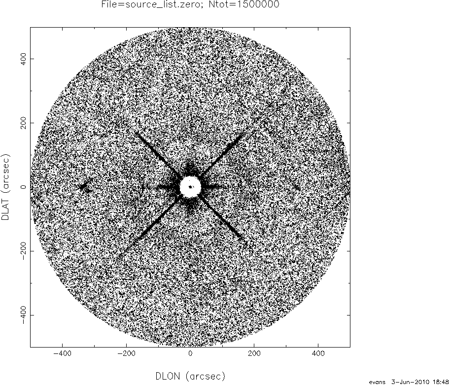 |
| Figure 1 - Example of a source-space image used to evaluate spike lengths and widths for coadds (images created with the multiframe pipeline). This particular image is for the magnitude 3.75-4.00 bin in Band 1, and is about 1000 arcseconds on a side.
|
Values of LS and WS are determined for each magnitude bin by inspection of these source-space images. LS and WS values are plotted versus mp, and a function is fit to them (Fig. 6 through 9). The functional form for LS was determined to be:
log10LS = aL * mp + bL
where 'aL' and ' bL' are tunable parameters, LS is in arcseconds, and mp is the parent star's magnitude. Note that in all cases, the fit tends to lie above the data points. This is because the linear fits were chosen to err on the side of overflagging; that is, the functions estimate the spike lengths to be somewhat longer than the actual spikes. The purpose of this is to ensure that real sources lying at the faint ends of the spikes are flagged as potentially contaminated. Since our initial evaluation of spike lengths were done using source-space images, the derived values are dependent on spurious sources being extracted from the diffraction spikes. At the faint end of the diffraction spikes, it is possible that no spurious extractions are being made, but there may still be a low level of flux capable of contaminating the photometry of real sources. Some minor overflagging is likely to occur because our parameters are tuned in this way, but this was done to ensure all affected sources were flagged.
To determine the optimal values of these parameters, a "test set" of 15 atlas coadds, spanning a range of ecliptic latitude, was used. These coadds were generated over a range of ecliptic latitudes and were constructed using the procedure used to create the atlas tiles for the WISE preliminary data release. The ARTID multiframe flagging algorithms were run on this test set, and adjustments were made to the parameters.
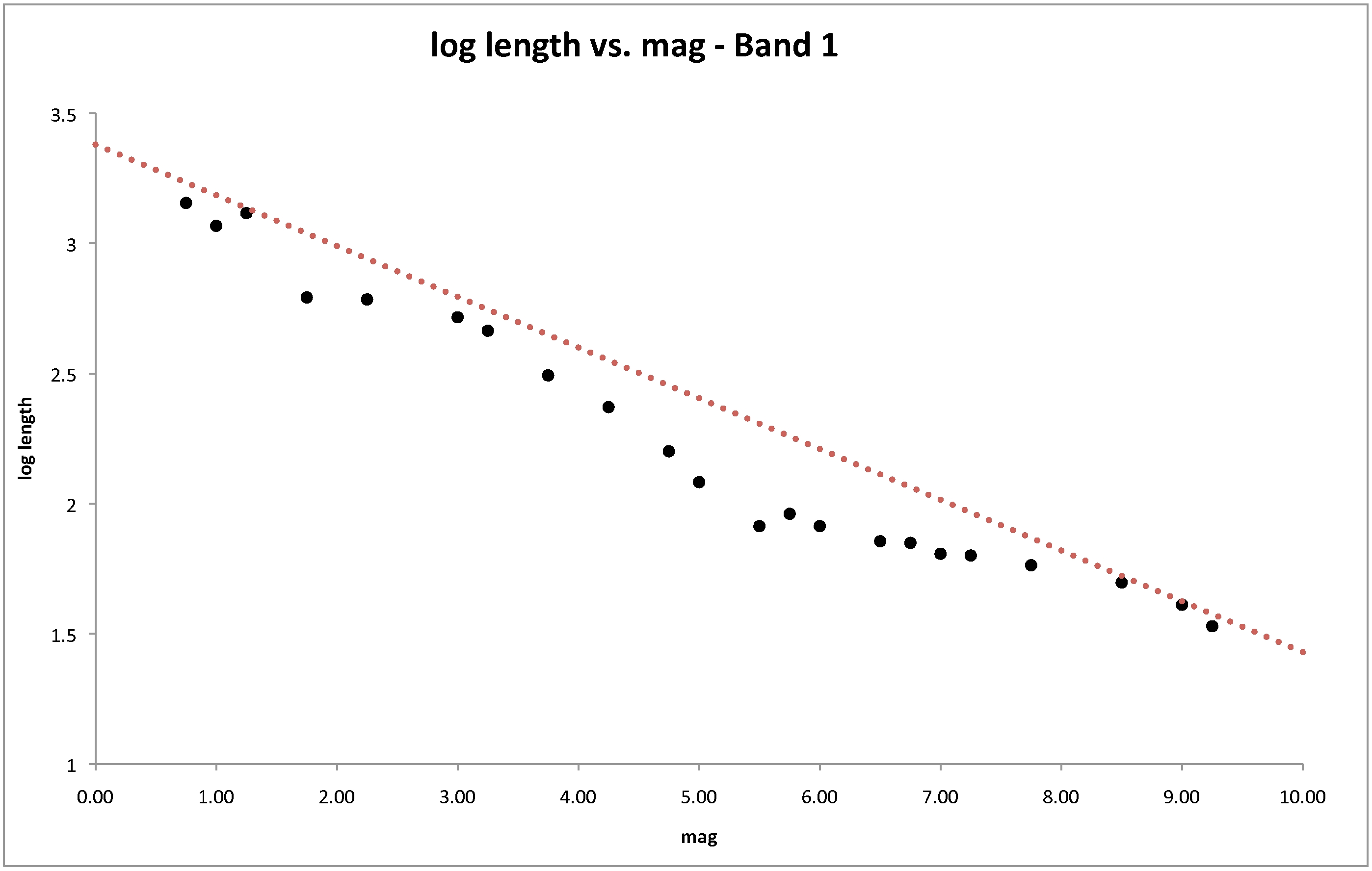 |
| Figure 2 - Plot of spike length (LS) vs. mp for Band 1. The black data points have been determined from the source-space images, as described in the text. The red dotted line indicates the fit, which is chosen to lie above most of the data points (see text for explanation).
|
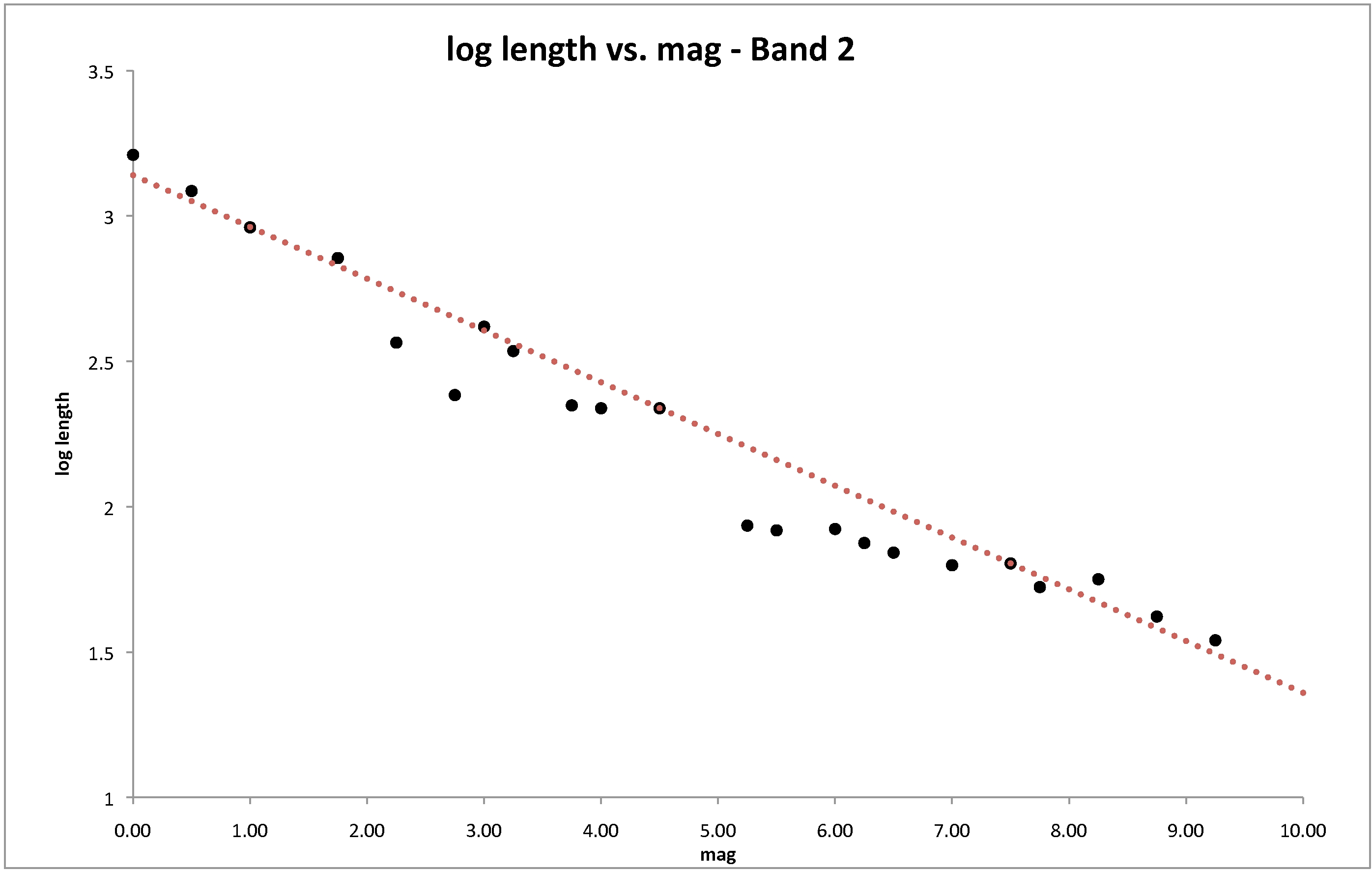 |
| Figure 3 - Same as Fig. 2, but for Band 2.
|
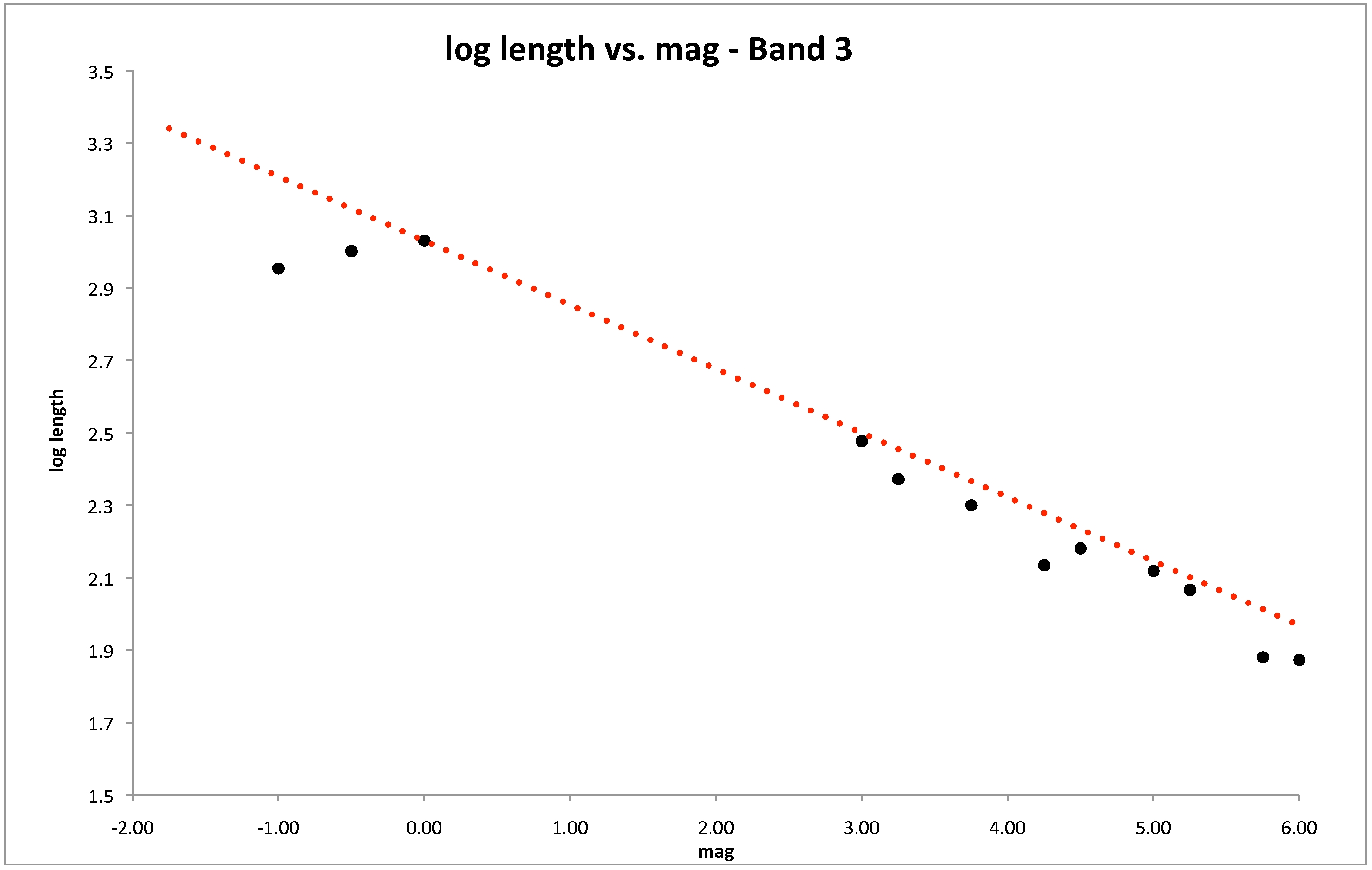 |
| Figure 4 - Same as Fig. 2, but for Band 3.
|
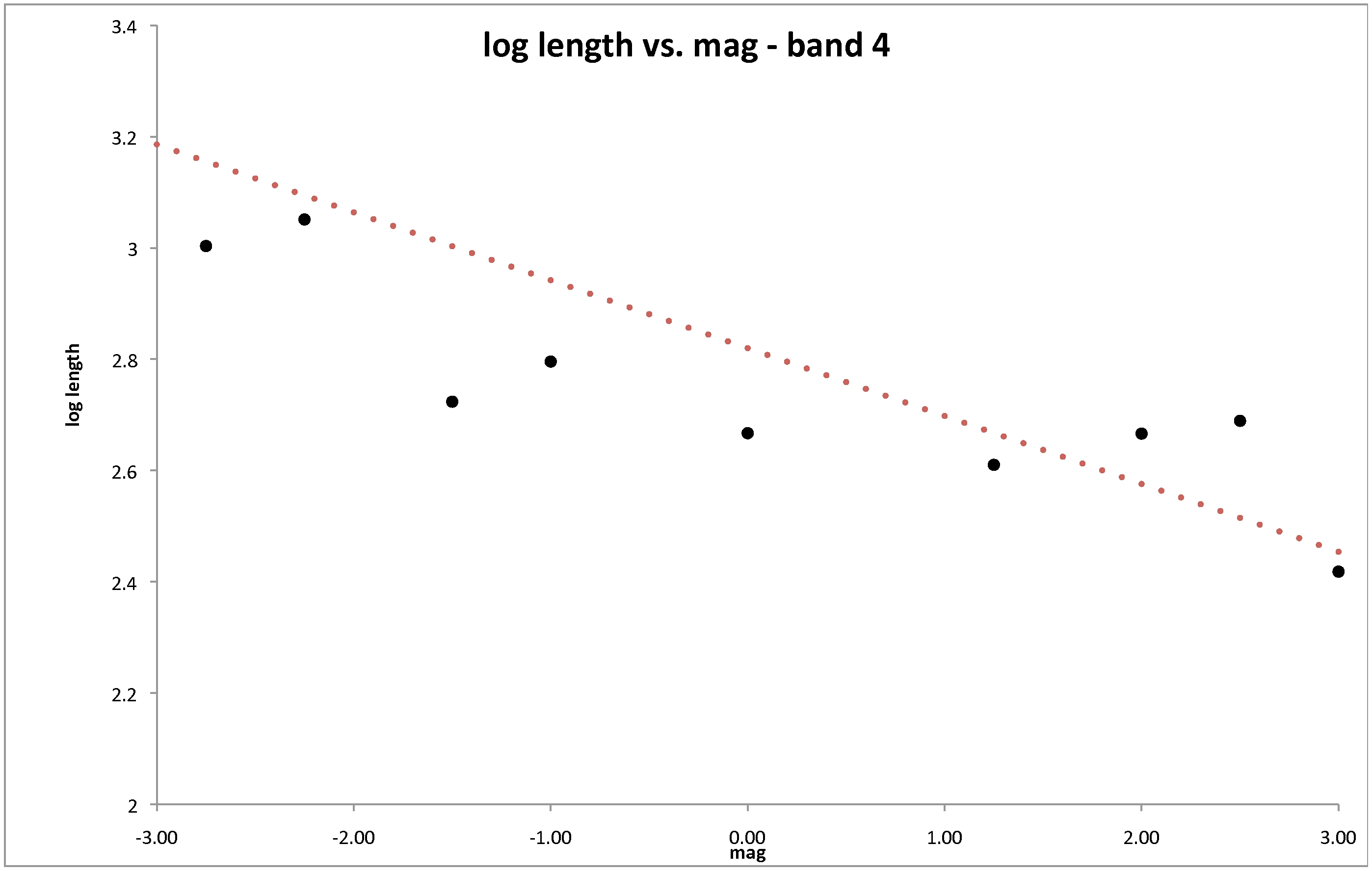 |
| Figure 5 - Same as Fig. 2, but for Band 4.
|
We also evaluate the parent star brightness at which spikes no longer appear, mthr_d, for each band. This is also done using the source space images. Spikes are considered to have disappeared once their lengths are well inside the radius of the halo. We list the final values of aL, bL, and mthr_d below in Table 3.
Table 3 - Length and Threshold Parameters for Multiframe Diffraction Spikes
| Band | aL | bL | mthr_d |
| 1 | -0.195 | 3.38 | 9.0 |
| 2 | -0.178 | 3.14 | 9.0 |
| 3 | -0.177 | 2.83 | 5.5 |
| 4 | -0.122 | 2.52 | 2.0 |
Spike widths, WS, were also determined by inspection of the source-space images described above. Values of WS were plotted vs. parent star brightness (mp), and fit to a function. Due to the large break in the relation at bright magnitudes, and the relative insensitivity in WS with respect to mp after the break, a step function was used, with the general form:
WS = aW; mp ≤ m1
WS = bW; m1 < mp ≤ m2
WS = cW; mp > m2
Like the values of LS, values of WS were also overestimated. This was primarily done to account for the width of a source in close proximity to a spike, possibly resulting in the overlap of the object's point-spread function with the spike, even though the extraction at the center of the source may lie outside the spike's formal width. Figures 10 through 13 illustrate the WS vs. mp dependences. Table 4 shows the parameters used for spike widths. Initial determinations were subsequently tuned through test runs of ARTID on a set of 15 atlas-type coadds. Adjustments were made to the parameters after inspection of the atlas tiles.
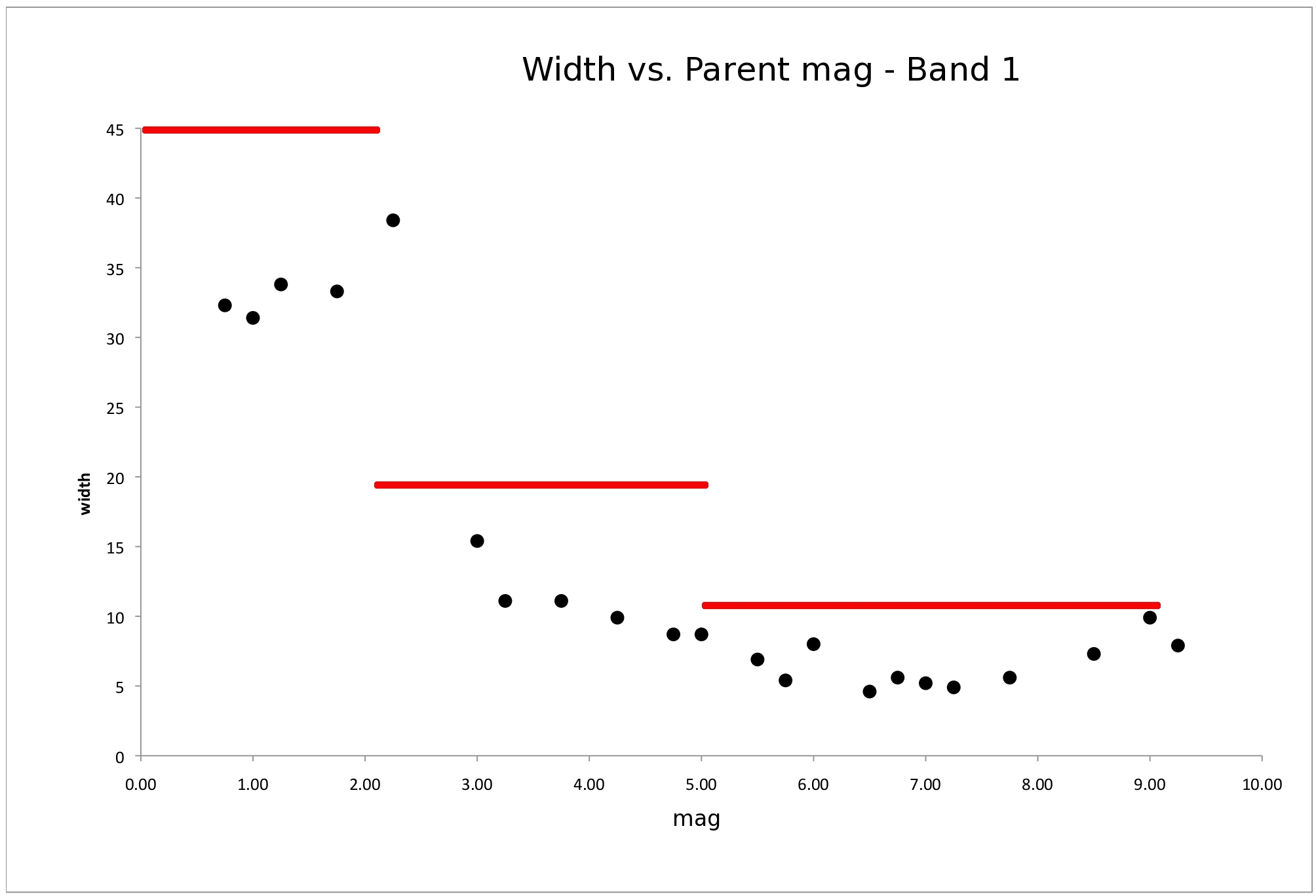 |
| Figure 6 - Plot of spike width (WS) vs. mp for Band 1. The black data points have been determined from the source-space images. The red lines indicate the step function used; they are intentionally overestimated as described in the text. Widths are given in arcseconds.
|
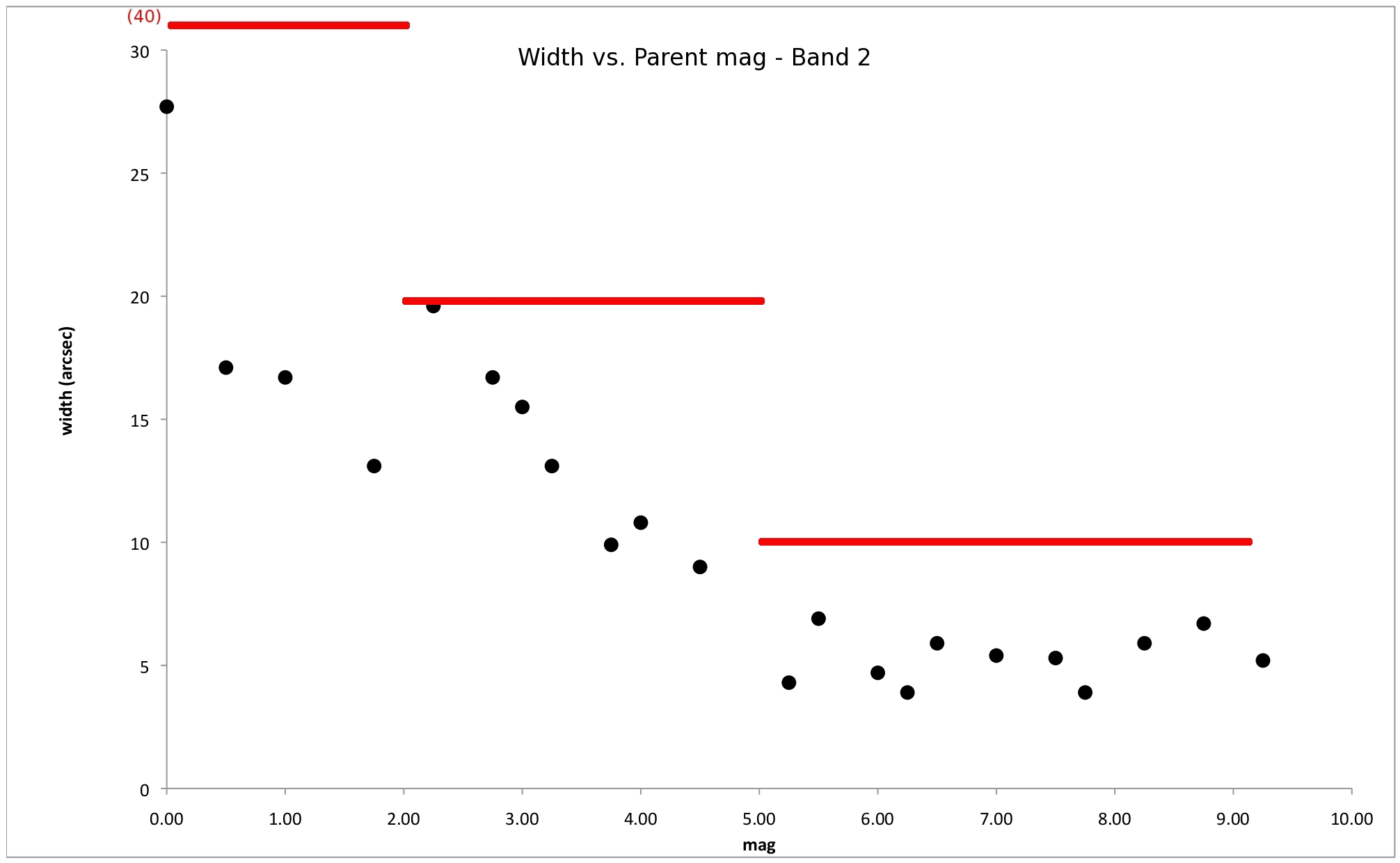 |
| Figure 7 - The same as Fig. 6 except for Band 2.
|
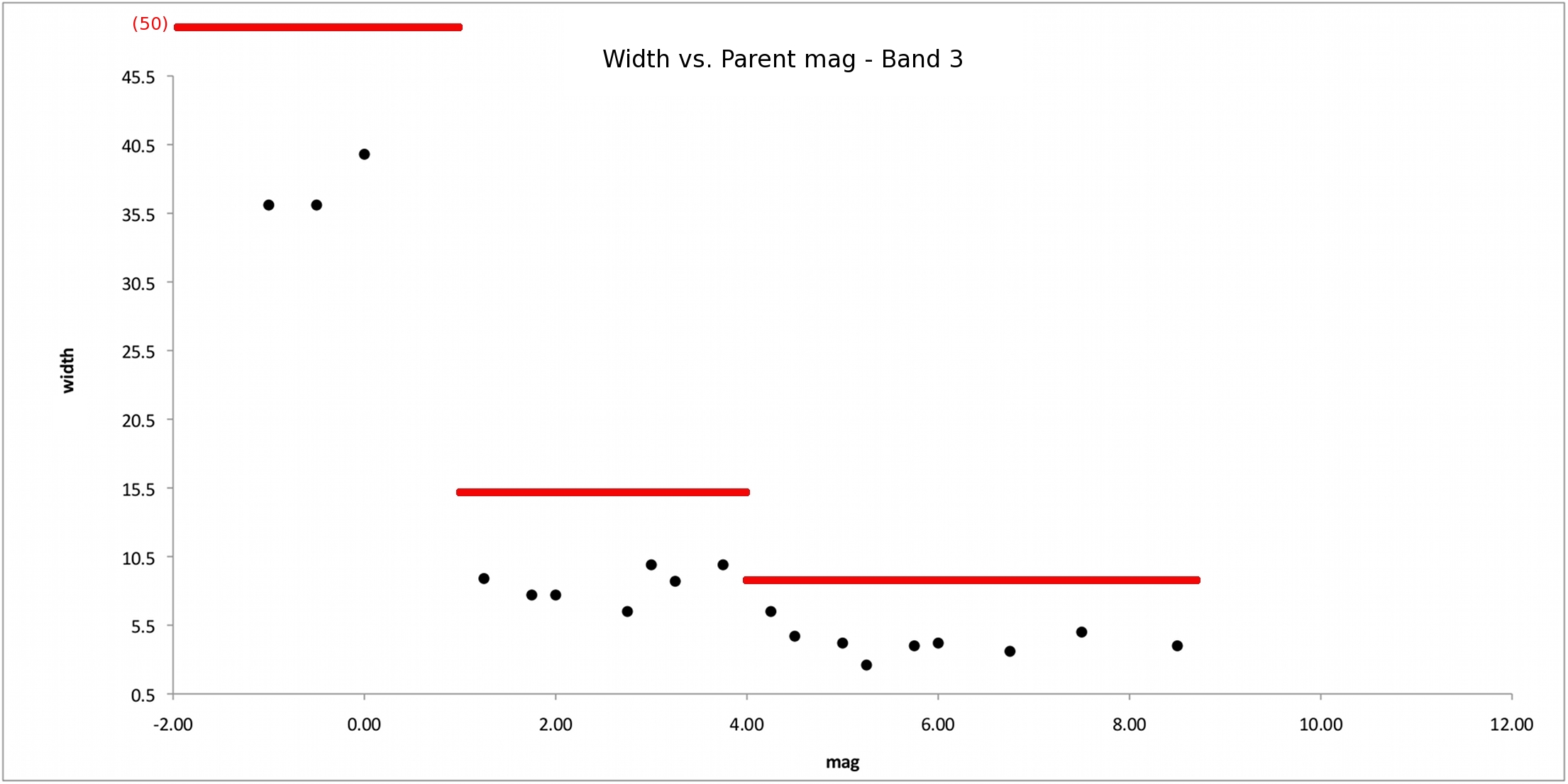 |
| Figure 8 - The same as Fig. 6 except for Band 3.
|
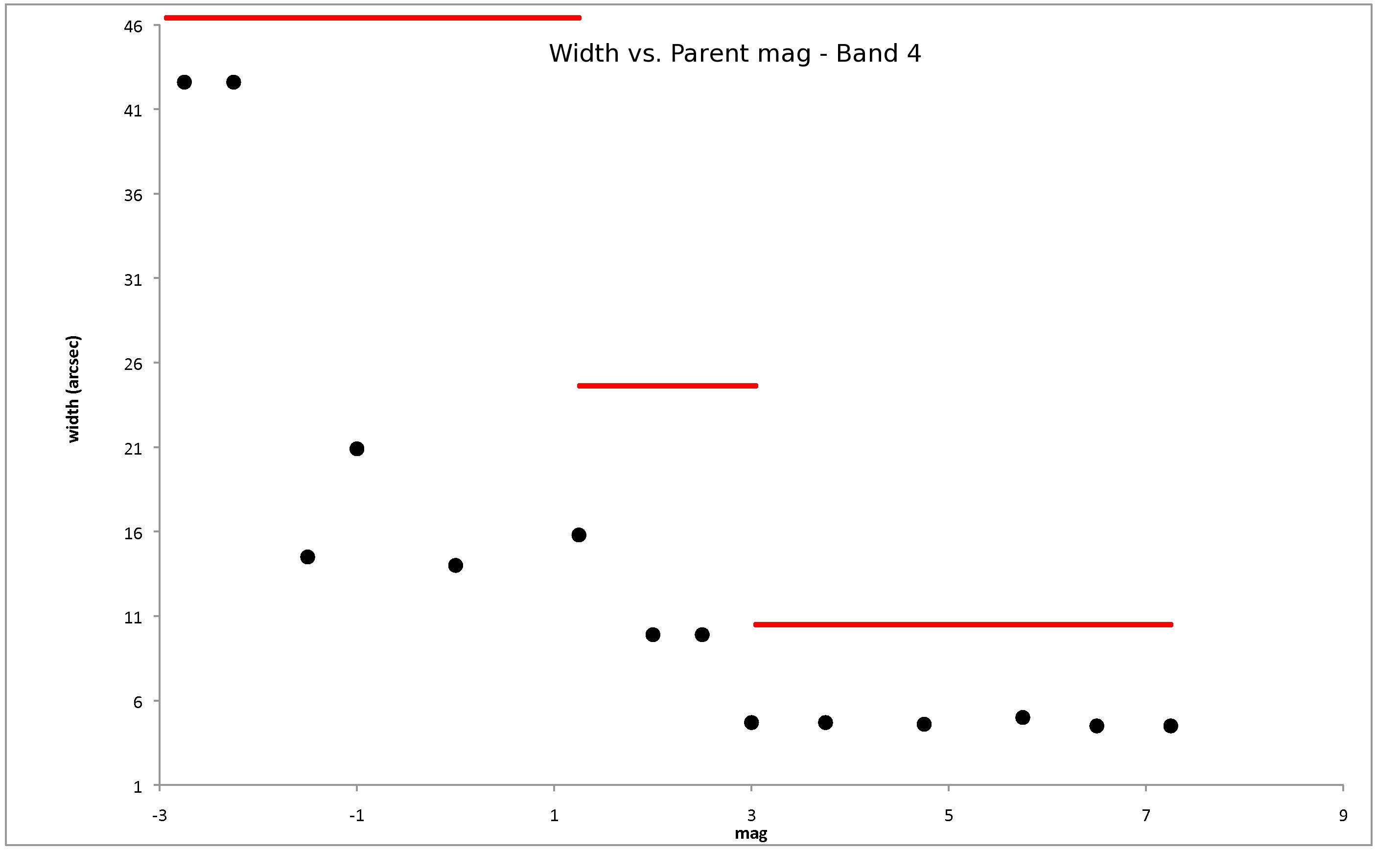 |
| Figure 9 - The same as Fig. 6 except for Band 4.
|
Table 4 - Width Parameters for Multiframe Diffraction Spikes
| Band | aW | bW | cW | m1 | m2 |
| 1 | 45.0 | 20.0 | 10.0 | 2.0 | 5.0 |
| 2 | 40.0 | 20.0 | 10.0 | 2.0 | 5.0 |
| 3 | 50.0 | 15.0 | 7.0 | 1.0 | 4.0 |
| 4 | 50.0 | 25.0 | 10.0 | 1.5 | 3.0 |
2. Spurious extractions vs. real and contaminated sources
In the multiframe flagging, a source is determined to be spurious or real/contaminated using a threshold, Δmspur_d. Given a magnitude of the source in question, ms, and a parent-star magnitude of mp, if ms &#gt; mp + Δmspur_d, then the source is flagged as spurious (i.e., if ms ≤ mp + Δmspur_d, the source is flagged as a real/contaminated extraction).
The difference compared to scan/frame processing is the incorporation of variable thresholds for differentiating spurious extractions from real sources that are contaminated by the artifact. Since diffraction spikes become fainter as they move farther out from the center of the parent star, the spurious-real threshold, Δmspur_d, will be a function of distance from the parent, rparent. Hence we derive functions relating Δmspur_d to r by examining the magnitudes of spurious extractions along the diffraction spikes of several stars spanning a range of brightnesses and ecliptic latitude. The procedure is outlined below.
Parameter determination:
In order to determine the functional dependence of Δmspur_d on rparent, we utilized a set of 15 atlas-type coadds created as a testbed for the multiframe ARTID module. A number of bright sources with diffraction spikes were selected, and the magnitudes of spurious extractions along the spike were plotted as a function of distance from the center of the parent star. The nature of the spurious extraction was verified by eye to ensure that no real sources were included. The Δmspur_d vs. rparent plots are shown in Figures 14 through 17.
For each band, a separate function relating Δmspur_d was determined, following the general form:
Δmspur_d = aspur * rparentbspur + cspur for Bands 1, 2, and 3
Δmspur_d = constant for Band 4
where aspur, bspur, and cspur are the parameters to be determined. The parameters are tuned not for the best fit (lowest residuals) to the data points, but to ensure that all spurious extractions are flagged as such. Therefore, the parameters are chosen so that the predicted value of Δmspur_d is lower at any given point along the spike, than the large majority of actual spurious extractions. This ensures that spurious sources are flagged as spurious, but has the side effect that some real sources will also be flagged as spurious. This is unavoidable, since there is no clear cut threshold where all spurious extractions lie on one side, and all real sources lie on the other. In this way, reliability of the source catalog is favored over completeness. Table 5 lists the parameters for spurious vs. real determination in each band. It should be noted that there does seem to be some mild dependence of Δmspur_d on ecliptic latitude. This dependence is only accounted for insofar as the parameters are tuned to ensure that all spurious sources at any ecliptic latitude is flagged as such.
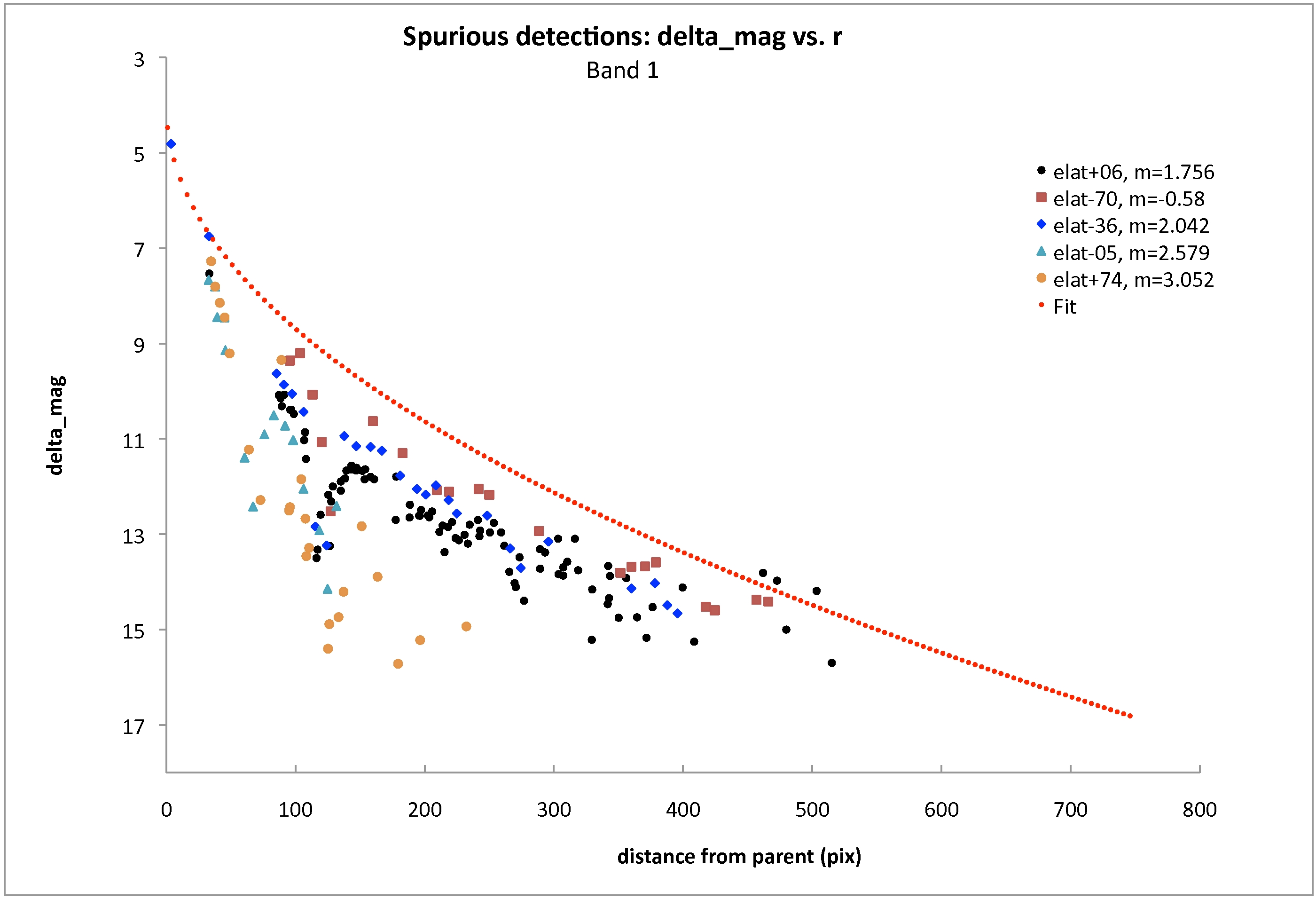 |
| Figure 10 - A plot of Δmspur_d for spurious extractions along the spikes of several bright parent stars (each symbol representing a different star), spanning a range of ecliptic latitudes in Band 1. A functional fit is also shown (red dotted line).
|
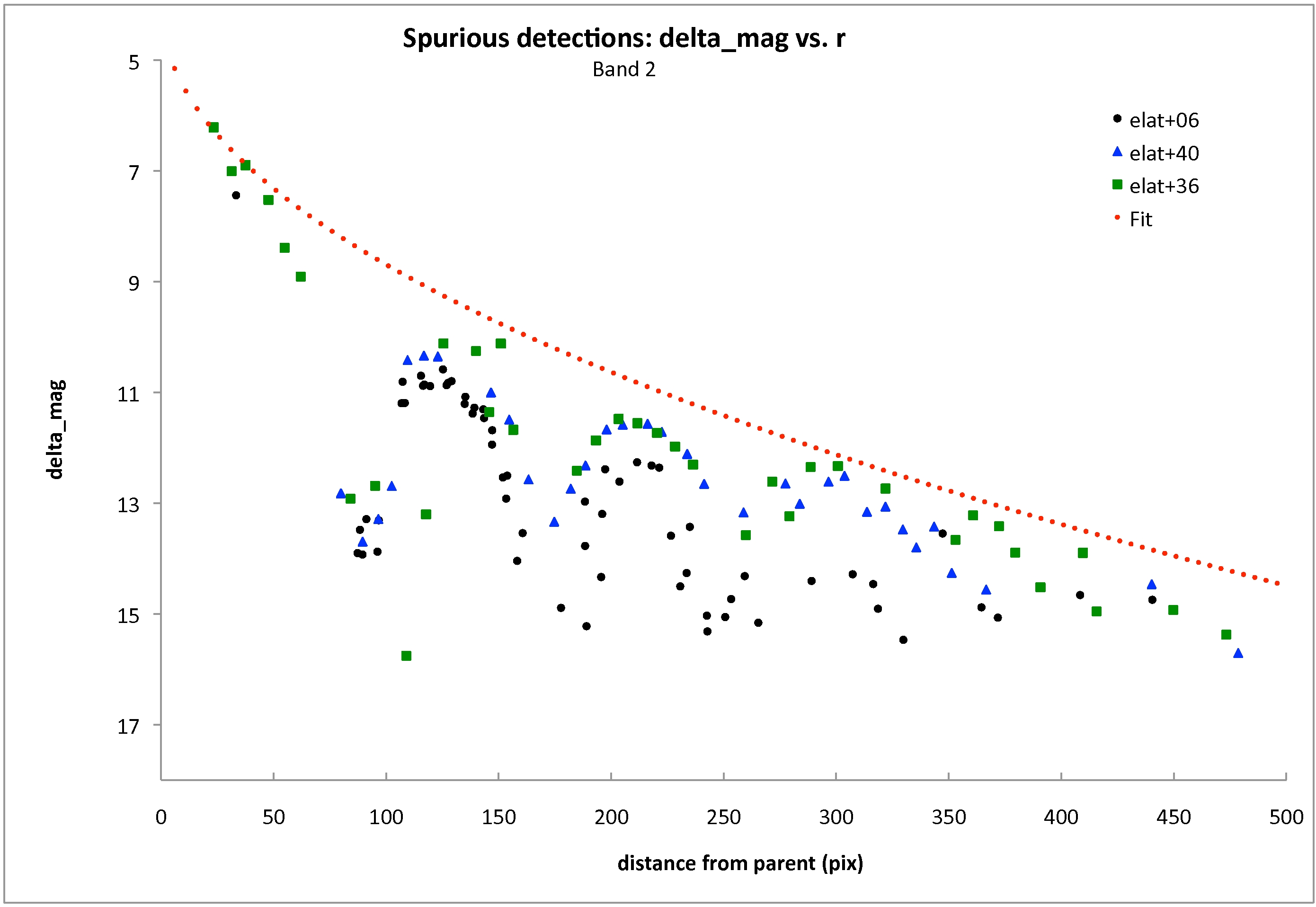 |
| Figure 11 - The same as Fig. 10 except for Band 2.
|
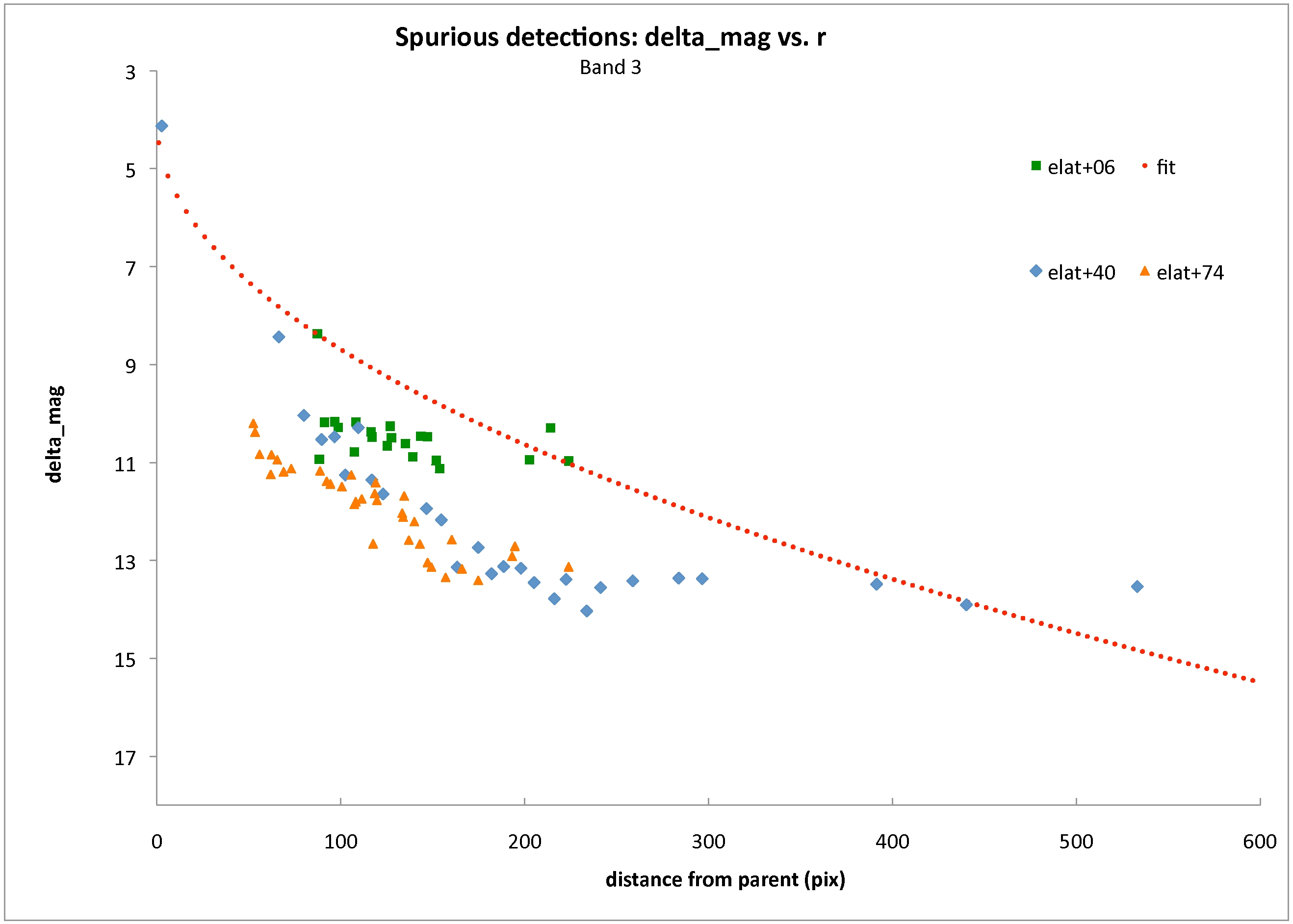 |
| Figure 12 - The same as Fig. 10 except for Band 3.
|
 |
| Figure 13 - The same as Fig. 10 except for Band 4.
|
Table 5 - Parameters for Spurious vs. Real Determination in Multiframe Diffraction Spikes
| Band | aspur | bspur | cspur | Band 4 Δm |
| 1 | 0.4 | 0.5 | 3.5 | N/A |
| 2 | 0.4 | 0.5 | 3.5 | N/A |
| 3 | 0.4 | 0.5 | 3.5 | N/A |
| 4 | N/A | N/A | N/A | 6.5 |
3. "Fanning" of Diffraction Spikes
At high ecliptic latitudes, diffraction spike behave differently in a coadded image (such as the Preliminary Release Atlas tiles). Due to the nature of the WISE orbit, regions near the ecliptic poles have high coverage (i.e., many single images are taken of the same piece of sky), and these single images span a range in position angle for any given piece of sky (i.e., the telescope is rotated differently with respect to the sky). Since the orientation of diffraction spikes are tied to the secondary support structure, and hence fixed with respect to the detector, the orientation of the diffraction spikes with respect to the sky will also vary from image to image. When coadded, this will result in the diffraction spikes taking on a "fanned" appearance due to the spread in observation angles in the single frames. Furthermore, the WISE image coadder incorporates outlier rejection which will eliminate artifacts in single frames when constructing the coadd (IV.6.a). This will tend to shorten the spikes compared the expected LS vs. mp relation. The method of flagging these diffraction spike "fans" essentially involves reading the position angle (PA; orientation) of the single frames which comprise the coadd and using the range in PA as the fan angle.
Cautionary Notes for Multiframe Diffraction Spikes
- Secondary spikes (any spikes other than the four most prominent diffraction spikes) are not flagged. The secondary spikes are most common in bright sources in Band 3 images.
- The brightest sources, particularly in Bands 1 and 2 (negative magnitudes) will generally have their spikes and halos underflagged (i.e., some spurious sources may not be flagged, or flagged as real/contaminated instead of spurious). This is because the functional forms and parameters were assessed using sources fainter than this. This is due to the fact that there are insufficient numbers of very bright sources available with which to build a source space image (see above for a discussion of parameter determination).
- Both spike lengths and widths have been intentionally overestimated. The purpose is to ensure that all extractions that are a result of, or affected by, artifacts are flagged as such. This also ensures that low-surface-brightness regions of the diffraction spike, where no spurious sources are extracted, but that may still contaminate photometry are captured by flagging. Thus, diffraction spike affected sources may be overflagged.
- Values of Δmspur_d are chosen to favor reliability of the WISE preliminary data release catalog completeness. Therefore, the parameters are chosen so that the predicted value of Δmspur_d is lower at any given point along the spike, than the large majority of actual spurious extractions. This ensures that spurious sources are flagged as spurious, but has the side effect that some real sources will also be flagged as spurious. This is unavoidable, since there is no clear cut threshold where all spurious extractions lie on one side, and all real sources lie on the other.
- Since outlier rejection in the WISE image coadder reduces the length of the diffraction spike in the final coadded image, lengths are overestimated, and overflagging may occur. The effect can be very significant, especially within a degree or two of the ecliptic pole, but is generally not important at ecliptic latitudes below 85 degrees.
ii. Scattered-light Halos (flag="h")
Bright sources are surrounded by a scattered-light "halo", essentially the outer portion of an object's point-spread function. This flux results in spurious extractions, and can, of course, also result in contaminated photometry for real sources. Analysis and characterization of halos were performed on processed multiframe data composed of several thousand atlas tiles.
1. Halo Radius
To determine a function relating the halo radius, rh, to the parent brightness, we plot the radius of the halo for several sources as measured from the altas coadds vs. the magnitude of the parent source, mp (Figure 18). The relation was determined to have the functional form,
log10(rh) = a * mp + b
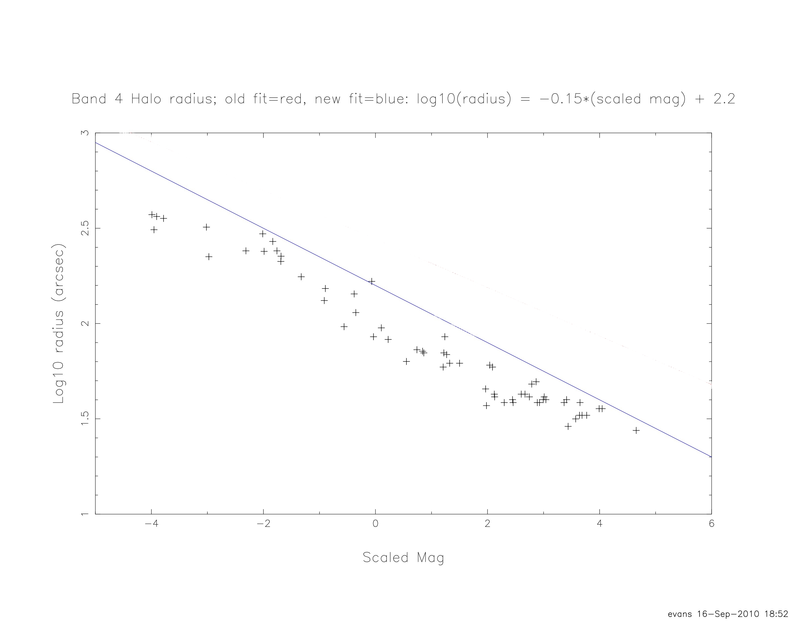 |
Figure 14 - Example (band 4) of halo radius, rh, vs. parent magnitude
for several sources in the atlas coadds. The blue line indicates the fit used.
|
We determine the optimum values for 'a' and 'b' in order to best predict a halo's radius. The fit overestimates the halo radius for the majority of magnitudes in order to ensure that all halo sources are flagged for all parent stars.The fitted parameter values are shown in Table 6. These values were subsequently tuned using test runs of ARTID on numerous atlas coadds.
Table 6 - Parameters for Multiframe Halo Radii
| Band | a | b |
| 1 | -0.144 | 2.76 |
| 2 | -0.113 | 2.49 |
| 3 | -0.157 | 2.48 |
| 4 | -0.150 | 2.20 |
2. Halo Real vs. Spurious Sources
In order to differentiate spurious sources (those that are extracted from, and exist purely due to, the halo) from real sources that lie inside and are contaminated by the halo, we define a magnitude difference, Δmspur_h. Consider an object which is extracted within the halo of the star to having a magnitude mh. If mh > mp - mspur_h, where mp is the magnitude of the parent star, is considered a spurious source. Equivalently, if the object in the halo is bright enough that mh < mp - mspur_h, it is considered a real and contaminated source.
To determine optimal value of mspur_h, as a function of the separation between the parent star and the halo source (d), we analyzed a number of sources from the atlas coadds.
To begin, we selected a set of atlas tiles that contained bright stars (m > 5), separating bands 1 and 2 from bands 3 and 4 because the bright stars in bands 1 and 2 are not the same sources as those in bands 3 and 4. We examined the coadd images for each band and tile in the set, and overlayed the complete coadd source list in that band and the list of sources already marked as "halo" objects in that band. We next adjusted the image stretch so that we could see as many faint (and moderately bright) sources as possible in the image,
so there was a clear difference between the diffuse halo emission and the background level; often we had to carefully find a balance between those two criteria.
For each of the brightest sources in the image, we selected the parent from the coadd [coadd_ID]-mfflag-3.tbl file
and marked it as such in a sorted copy of that file. We then examined each individual source in the halo region on the image and determined if it had the correct flag value. The method we used to determine the "correct" flag value was as objective as possible under the circumstances: we decided if the marked source is obviously a real source, i.e. it lies on top of a distinct local flux maximum,
or obviously a false source, i.e. it lies on top of an area of confused, bright diffuse emission quite close to the parent or an area without any apparent source detection at all. If we felt we could not clearly determine the correct flag value,
we ignored the source so the results would be as reliable as possible. This method results in a selection bias towards finding the real sources, since they are more obvious to the eye.
Below the parent source data, we added all the sources from the same file that were not marked as halo objects
but which we believed should have been flagged, and appended the correct cc_flags value to the data ('H' or 'h' in the correct band's character). We did the same for the sources that were marked as halo objects
but that we believed should have been flagged, and appended the correct cc_flags value ('0' in the correct band's character). We added the sources that were marked as real or spurious halo sources ('h' or 'H', respectively)
but which we thought should be marked as the opposite type, and again appended the correct cc_flags value to the data.
And finally, we added some sources with flags that we agreed were correct.
We performed this analysis for as many parents in each coadd as possible, in order to get as large a range of parent magnitudes as possible. However, we concentrated on the brightest parents because the algorithm differentiating between the
spurious and real halo sources should not depend on the parent magnitude; it only depends on the band, the distance between the parent and halo source, and the magnitude difference between the same.
After gathering all the results from this analysis, we ran them through a program that calculated the distance and magnitude differences
between each parent and its corresponding halo sources. We then performed fits to this data, deriving a functional form for the relation:
Δmspur_h = a * log10(d) + c,
Where 'a' and 'c' are the derived parameters. using different marks for the real and spurious halo sources as determined by the procedure above. We then drew a line in the region of overlap between the real and spurious sources,keeping it as low as possible (to put most of the real sources above the line) while still leaving the bulk of the spurious sources below the line. This skews toward keeping as many sources as legitimately possible marked as real, not spurious, sources. The derived values of the parameters are shown in Table 7.
In the following figures (19 through 22), the green circles in the plots indicate real halo sources, and the red triangles indicate spurious sources. The open vs. filled marks only indicate different sets of images that were examined at different times;
both sets of images apparently follow the same relationship between Δm and log10(d).
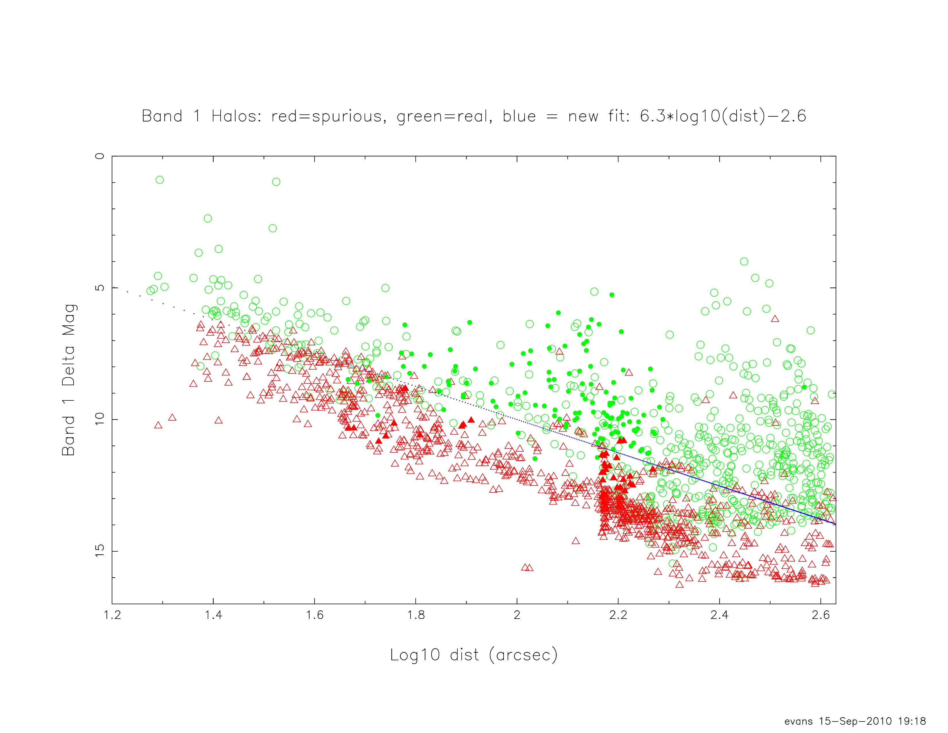 |
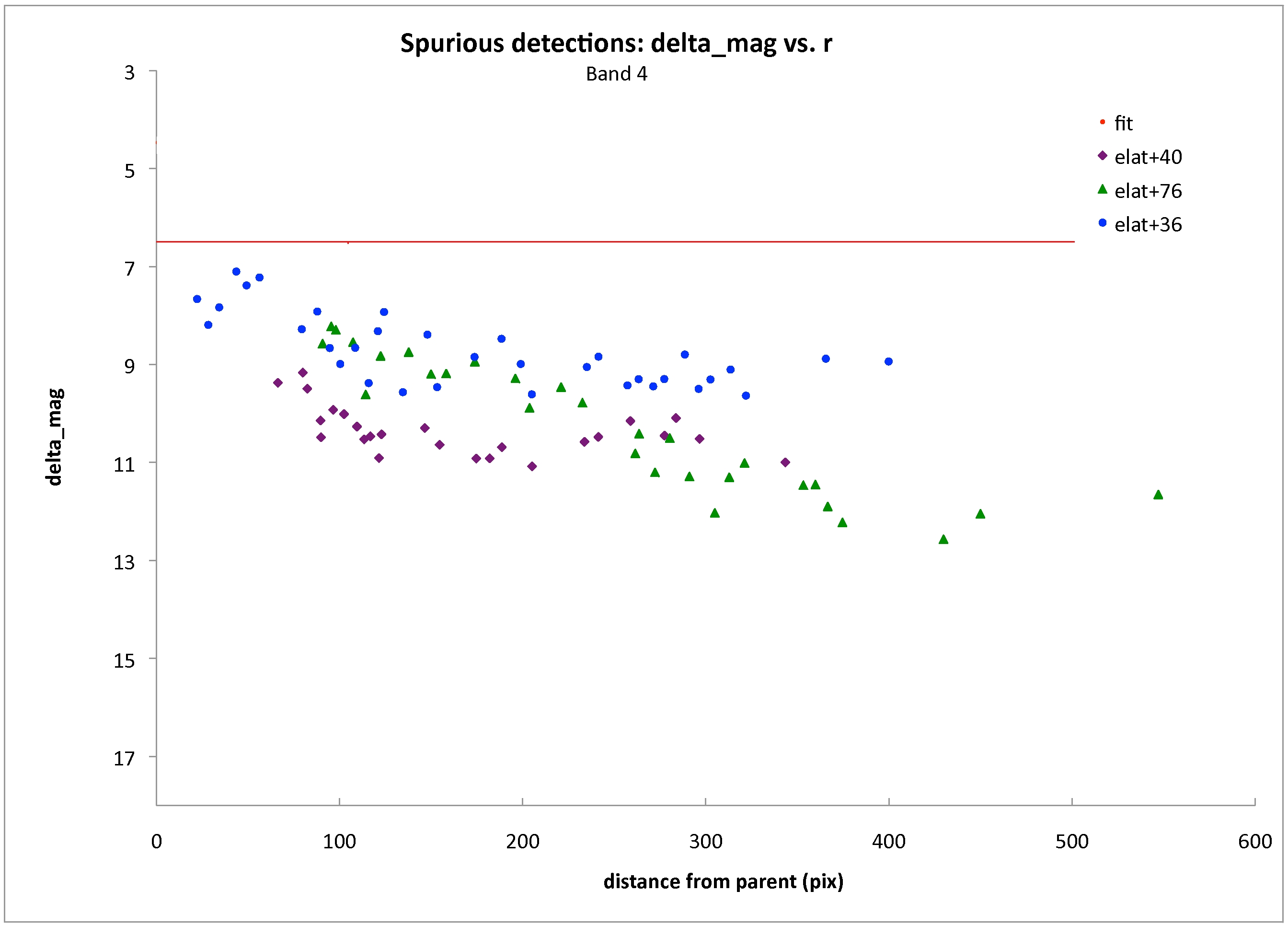
Figure 15 - Δm (parent - source magnitude) vs. distance
from parent, d, for sources in the coadds, Band 1.
|
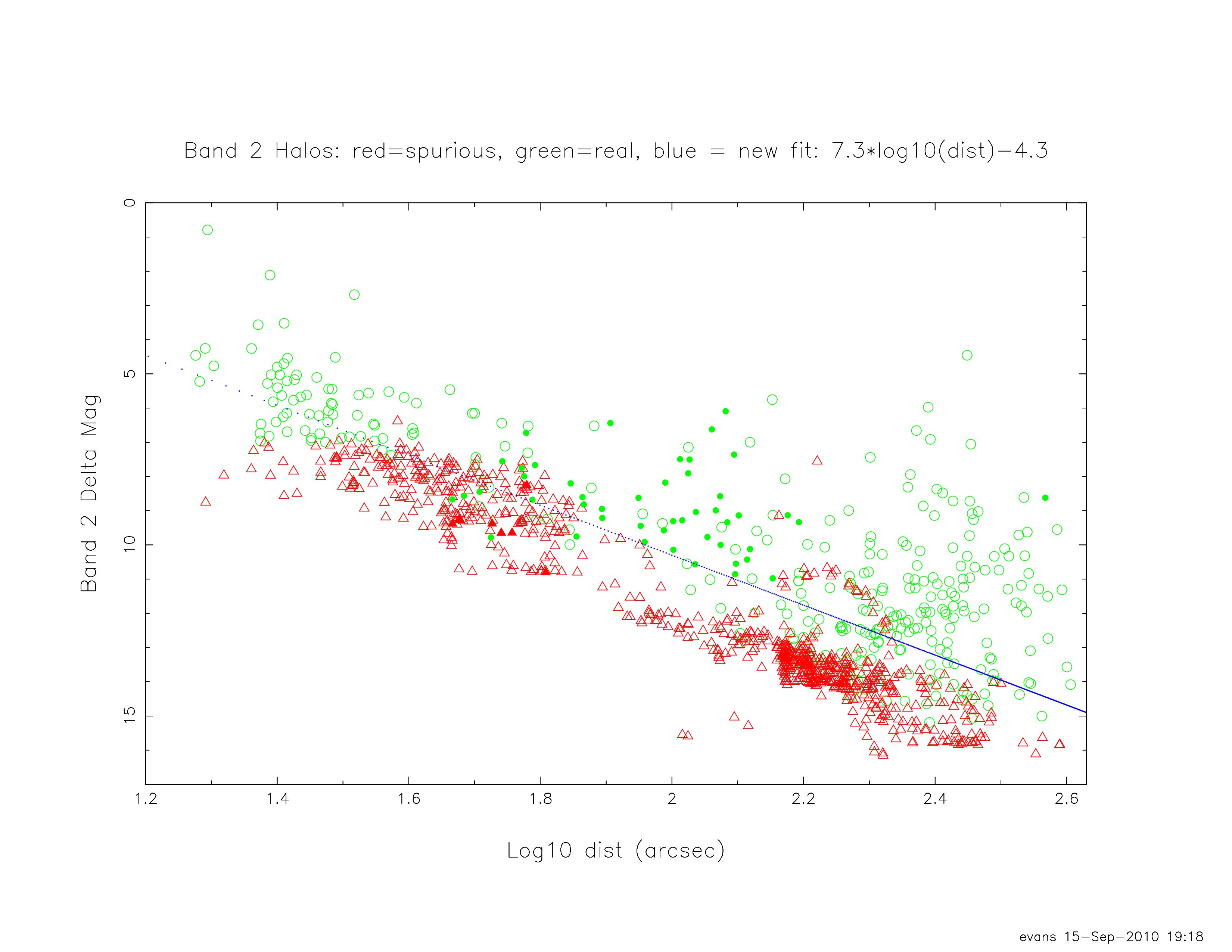 |
| Figure 16 - Same as Figure 15, but for Band 2.
|
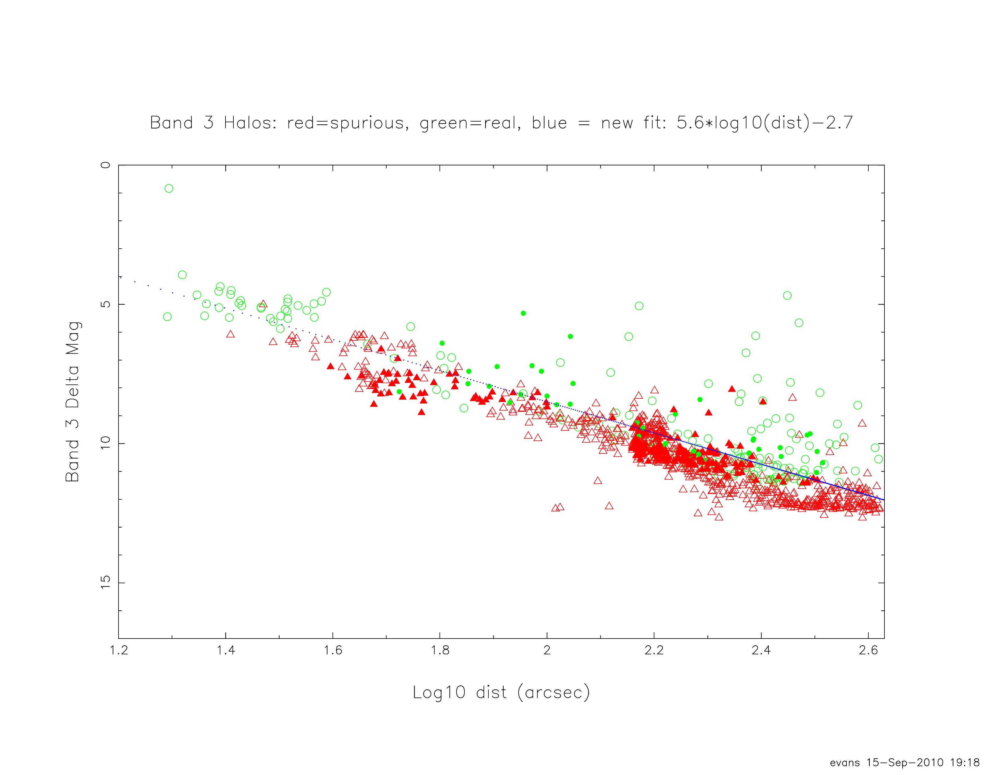 |
| Figure 17 - Same as Figure 16, but for Band 3.
|
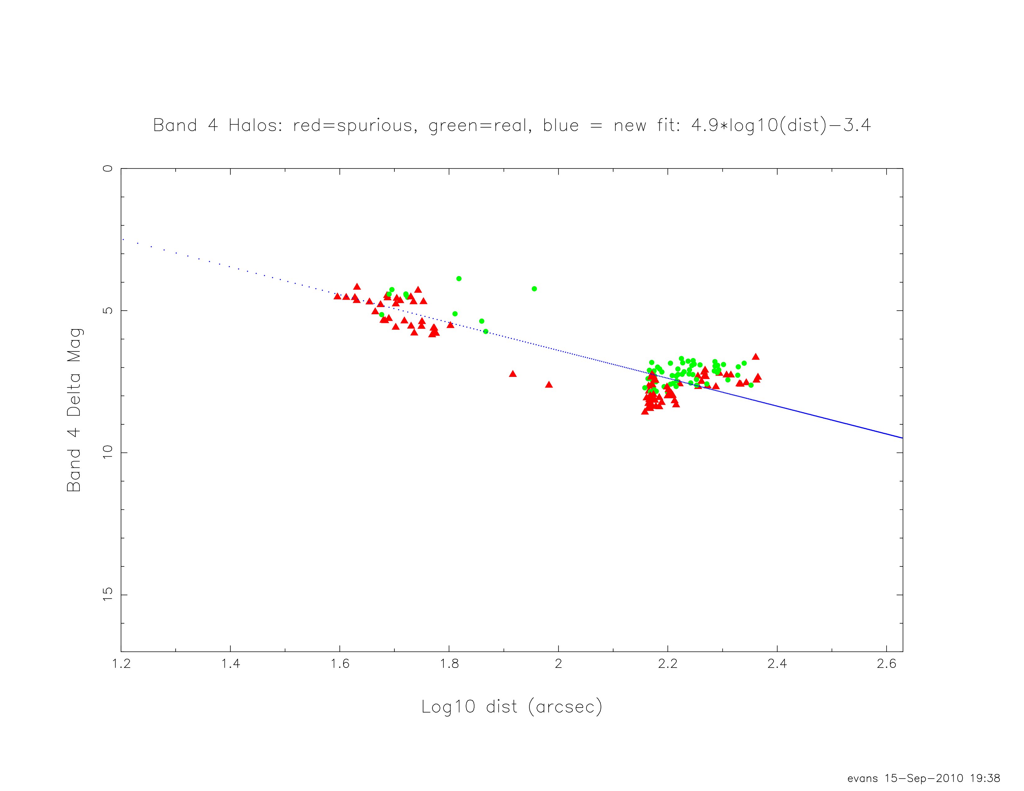 |
| Figure 18 - Same as Figure 16, but for Band 4.
|
Table 7 - Real vs. Spurious Source Parameters for Multiframe Halos
| Band |
a |
c |
| 1 |
6.3 |
-2.6 |
| 2 |
7.3 |
-4.3 |
| 3 |
5.6 |
-2.7 |
| 4 |
4.9 |
-3.4 |
iii. Optical Ghosts (flag="o")
Since optical ghosts are always located in the same position relative to a bright parent star, they will appear, quite prominently, in coadded images. Optical ghosts in the multiframe version of ARTID are treated in much the same manner as single-frame flagging. The major changes are noted below. The definition of the parameters remains the same as single-frame ghost flagging, however their values do change. For a description of the parameters, refer to single frame ghost flagging.
Changes in coadd ghost flagging that were implemented include:
- The addition of a Band 1 ghost. In single-frames, the ghost in Band 1 was generally not visible, because it was a low-surface-brightness artifact, and the parent stars which were bright enough to host ghosts encompassed the ghost inside the halo. In coadded images, the Band 1 ghosts begin to appear for fainter parents.
- Since the coaddition of single-frames results in low-surface-brightness parts of the ghost becoming more visible in the coadds, the ghosts increase in size by a small amount. Hence, values of Rghost change. Values of mthr_o and Δmspur_o also change do to fainter ghosts becoming more detectable in coadded images.
As with single-frame ghost flagging, parameters for ghosts include the radius of the circular region inside which sources are flagged (Rghost). The positional offset from the center of the parent star, Δx and Δy, are also parameters. Additional parameters are mthr_o, the parent star magnitude at which ghosts appear, and Δmspur_o, the magnitude threshold used to differentiate spurious extractions on the ghosts from real sources whose photometry is contaminated by the ghost. The value of mthr_o was determined by inspection of a 20-40 of bright sources and their ghosts taken from the atlas-type coadd test set (described in the Diffraction Spike section above), over a range in brightness. Values of Δmspur_o were assessed in a manner similar to the single-frame determination, but using stars from the atlas coadd test set. The final values of the parameters are listed in Table 8, with positional offsets and Rghost given in arcseconds (as opposed to single-frame pixels which were used in Table 2).
Table 8 - Ghost Parameters Multiframe Flagging
| Band | Δx | Δy | Rghost | mthr_o | Δmspur_o |
| 1 | 313.5 | 0.0 | 35.8 | 2.0 | 12.0 |
| 2 | 313.5 | 0.0 | 35.8 | 4.5 | 9.0 |
| 3 (1st ghost) | 0.0 | -566.5 | 75.6 | 4.0 | 6.5 |
| 3 (2nd ghost) | 0.0 | -1130.3 | 123.8 | -1.6 | 7.5 |
| 4 | 0.0 | -566.5 | 89.4 | 1.0 | 6.5 |
iv. Persistence (Latent Images)
In the V3.5 WISE coadd (MFF) pipeline, the radius for
short-term latent flagging is set at 3 pixels for the HgCdTe arrays and 100
arcsec for the Si:As arrays. Short-term latents, especially the large
ones seen in the W3/W4 arrays, tend to add constructively in the coadded
images and can be seen somewhat further downstream of their parent sources
than in the single frames except in areas near the ecliptic poles.
Long-term latents are not flagged in the coadd
pipeline. As the scan angle changes over time in regions other
than the ecliptic plane, long-term latents will tend to
spread out and not constructively stack causing them to be rejected
as outliers. Their presence is shown in the coadd coverage images as the
many sets of contiguous pixels in which there are diminished coverage.
Table 9 - Multiframe Latent Parameters
| Band | Δmspur | Parent Flux Density(Jy) |
| 1 | 7.0 | 0.2 |
| 2 | 7.0 | 0.3 |
| 3 | 8.5 | 1.1 |
| 4 | 7.0 | 1.65 |
Last update: 2012 January 19
Previous page Next page
Return to Explanatory Supplement TOC