|
(Eq. 1) |
The advantages of doing the detection simultaneously at multiple bands are:
1. Increased sensitivity to weak sources due to the fact that detection is based on the stack of images at all bands.
2. No separate bandmerging step is required, thus avoiding the ambiguities which can occur when trying to associate sources in different bands in the presence of confusion.
3. The higher resolution data at the shorter wavelengths can guide
the extraction at the longer wavelengths where the resolution is poorer.
The multiband estimation process represents a departure from the traditional procedure, employed in such software packages as DAOPHOT ( Stetson 1987 PASP, 99, 191) and SExtractor ( Bertin & Arnouts 1996, A&AS, 117, 393), in which detection and characterization are carried out one band at a time. Another motivation for developing new source extraction algorithms is that currently available packages operate on a single regularly-sampled image rather than a set of dithered images. The procedures employed in MDET and WPHOT are optimized for the latter case. MDET is based on an algorithm which is optimal for the detection of non-blended point sources in the presence of additive Gaussian noise, given an observed image or a set of observed images (spatially dithered and/or at one or more bands). Our implementation extends its applicability to crowded fields.
Inputs to MDET include the coadded images and bad pixel masks, generated by the AWAIC module, and a detection threshold representing the assumed lower cutoff in signal to noise ratio. In the Scan/Frame Pipeline for the Preliminary Release, that threshold was set at 5 sigma. The output is a set of source candidates, with equatorial positions, listed in order of decreasing signal to noise ratio. Note that although coadded images are used as input, they are used in such a way that the result is essentially the same as what would have been produced by optimally combining the dithered focal-plane images themselves.
The starting point for the detection step is the measurement model for an isolated point source, assumed to be at location s and to have flux fλ in the waveband denoted by index λ ; it can be expressed as:
|
|
(Eq. 1) |
It is advantageous to estimate the background, bλi ahead of time (we use median filtering with a window size appropriate to the characteristic spatial scale of background variations) and subtract its contribution, so that the measurement model may be rewritten:
|
(Eq. 2) |
Based on the measurement model expressed by Equation 2, the source detection procedure involves comparing the relative probabilities of the following two hypotheses at each location, s, within a predefined regular grid of points on the sky:
Hypothesis (A): s lies on blank sky at all wavelengths
Hypothesis (B): s represents the location of a source whose flux densities are the most probable values, denoted by f^λ.
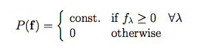
To compare these hypotheses requires knowledge of f^λ, which we obtain by maximizing the conditional probability, P(f | ρ), with respect to f, where f is a vector whose components are the set of fλ, and ρ is a vector whose components are the set of pixel values, ρλi, in the vicinity of s. The conditional probability itself is given by Bayes' rule, i.e.,
|
(Eq. 3) (Eq. 4) |
and P(f) represents our a priori knowledge about possible flux values. Our most important piece of knowledge in that regard is that flux is positive. With the exception of the positivity, however, we will assume that we have no prior knowledge of flux or the spectral variation of flux, in order to avoid introducing any color biases in the source detector. We can thus express P(f) as:
|
(Eq. 5) |
The remaining quantity, P(ρ), in Equation 3, represents a normalization factor. The maximization of P(f | ρ) then yields:
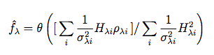
|
(Eq. 6) |
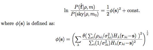
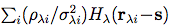
where Hλi = Hλ(rλi - s) and θ(x) represents a function which is equal to its argument, x, if the latter is nonnegative and 0 otherwise. The summations in Equation 6 are over all pixels within a predefined neighborhood of s.
With a further application of Bayes' rule, we can now express the probabilities of hypotheses (A) and (B), above, as:
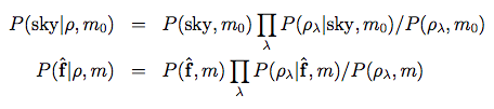
| (Eq. 7) (Eq. 8) |
where m0 represents the sky-only model corresponding to hypothesis (A), and m represents the model corresponding to hypothesis (B), based on Equation 2.
The likelihoods P(ρ | sky, m0) and P(ρ | f^λ, m) are given by:
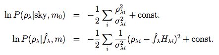
|
(Eq. 9) (Eq. 10) |
Assuming that we have no prior knowledge about the possible presence or absence of a source at s, all of the other factors in Equations 7 and 8 may be regarded as constants for present purposes, and we can thus express the probability ratio (source/sky) as:
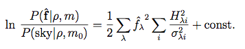
|
(Eq. 11) |
Substituting for f^λ using Equation 6, we can express this probability ratio as:
|
(Eq. 12) (Eq. 13) |
in which we have replaced Hλi by its more explicit form.
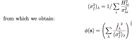
From Equation 12, maxima in φ(s) correspond to maxima in the (source/sky) probability ratio, and hence an image formed by calculating φ(s) over a regular grid of positions, s, would be a suitable basis for optimal source detection. It is apparent from Equation 13 that such an image represents a quadrature sum of matched filters at the individual wavelengths, with appropriate normalization. The noise properties of such an image can be assessed by expressing φ(s) in terms of the a posteriori variance of f^λ, given by:
|
(Eq. 14) (Eq. 15) |
It is readily shown, from Equation 15, that the standard deviation of
To summarize, the calculation of the optimal detection image from a
set of multiwavelength observations involves simply the quadrature sum
of the matched filter outputs (normalized in units of sigmas) at the
individual wavelengths, as illustrated in Figure 1.
Detection then consists of searching for local maxima which exceed a
specified signal-to-noise threshold in this image.
In the above derivation, the assumption was made that
the instrumental responses of adjacent sources do not overlap. Although
all matched filters are subject to this limitation, the situation can be
more acute in the case of the multiband matched filter since images are
being combined at multiple spatial resolutions. For the limited range
of spatial resolution in WISE (a 2:1 ratio in FWHM between
W4 and W1) one would not expect any serious problems since, for example,
closely-spaced (but distinct) peaks in the W1 image would normally produce
local maxima in the combined image even if superposed on the wings of a
broader W4 peak. However, if
a source is present in W1 only, and a neighboring source is present in
W4 only (or vice versa), the two sources could be blended into a single
peak in the combined detection image even though they produced separate
peaks in their respective single-band images.
These effects are overcome by supplementing the set of multiband
detections with the results of single-band detections. By doing this,
we maintain the increased sensitivity of multiband detection while
not missing any detections due to cross-band blending effects.
The central operation in MDET is the calculation of the detection image, given
by Equation 13. It is fortunate that the majority of the
computations involved in this step (specifically, summations over the data
pixels with weighting factors derived from the PSFs) are essentially the
same as those used
in the calculation of the estimated sky brightness distribution at each
band, performed by the WSDS image coadder,
AWAIC.
Therefore we can save a considerable amount of computation time by making
appropriate use of that module's output. Specifically, the
expression
Expressing the detection image, φ(s), in terms of the
coadded image, Iλ(s),
using Equation 13 we thereby obtain:
where bλ(s) represents the slowly-varying sky background and
σλ(s) its local standard deviation.
We estimate bλ(s)
via median filtering of the coadded image using a
window size, wλ, chosen to be somewhat smaller than
the assumed (a priori) minimum scale of sky background variations.
Our standard adopted value of
wλ for the Preliminary Release was 400 coadd
pixels, i.e., 550 arcsec. The sky background is estimated at a grid
of points spaced by
wλ and interpolated using a Gaussian smoothing
kernel. The corresponding local standard deviation of background noise,
σλ(s), is then estimated from the residuals
between the coadded image and the slowly-varying background using the
difference between the mode and 16% quantile of the histogram of those residuals.
So the multiband detection procedure is:
1. Estimate a slowly-varying sky background and standard deviation of
background noise at each wavelength, as described above.
2. Subtract the estimated background from each coadded image.
3. Calculate the optimal matched filter at each wavelength
(represented by an individual term in square brackets in Equation 16.
4. Zero out negative pixel values in each of the single-band
matched filter images.
5. Combine the resulting single-band images in quadrature to
produce a detection image in units of sigma (the local standard deviation
of noise).
6. Locate all local maxima in the detection image, to an accuracy
corresponding to the pixel size of the coadded image grid.
7. List the positions (RA and Dec) and strengths (i.e., SNR values)
of all local maxima which exceed the desired detection threshold in sigmas,
in order of decreasing SNR. In the Scan/Frame pipeline for the
Preliminary Release, a detection threshold of 5σ was used.
8. Repeat the detection procedure for each band individually
and supplement the multiband source list with any single-band detections that
were missed in the multiband step. The criterion for the inclusion of
a single-band detection is that the distance between it and the nearest
source on the multiband source list should exceed a critical distance,
rcrit. The latter corresponds to the minimum distance between
distinguishable peaks on the matched filter image for the band in
question, for which an appropriate value is 1.3 times the FWHM of the
PSF in that band.
In regions of high source density, such as the Galactic Plane, the effects
of unresolved background sources act like an additional
stochastic component in the measurement model for our sources of interest
(the latter being defined as point sources spatially resolvable either
directly by the measurement system, or by subsequent processing). This
stochastic component, referred to as "confusion noise" is automatically
taken account of by the above procedure in which we estimate the
local background noise on the fly. Specifically, the estimated background
noise increases in confused regions, and since we
regard the detection threshold as being constant in terms of SNR,
we are effectively raising the flux density limit in such regions.
Stars with saturated cores produce "craters" in the detection image, and
hence a ring of spurious source peaks. Such cases are identified by looking
for groups of contiguous saturated pixels in the bad-pixel mask. The
grouping is done using an image segmentation routine, and the source
location is then taken as the centroid of the group. The effective
radius of the group of saturated pixels is calculated using the
2nd moment, and this value, rsat, is passed to
the WPHOT module to facilitate appropriate choices of
fitting radii for profile-fitting photometry in those cases.
The local standard deviation of the background, σλ(s),
is raised in the vicinity of the saturated star in order to suppress
spurious source peaks due to complex structure in the wings of the PSF.
This is done by estimating the standard deviation of pixel values in
a series of concentric annuli surrounding the star.
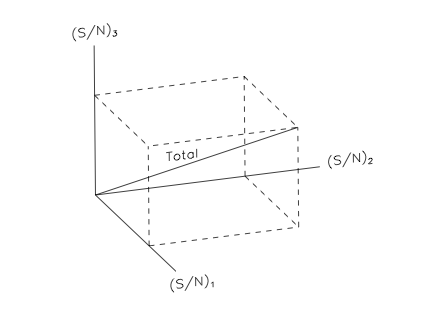
Figure 1 - Combining matched filter images at several wavelengths.
In this
illustration, matched filter signals (in units of signal to noise ratio,
SNR)
from three separate bands are combined in quadrature to produce the
total response.
This detection algorithm is similar to one proposed by
Szalay et al. 1999 AJ, 117, 68,
often referred to as the "chi squared" method. The central operation,
in both cases, is a quadrature sum of matched filter images.
An important difference between the two procedures, however, is the
fact that in MDET we threshold the matched filter images at zero before
squaring and combining, thus avoiding the contaminating effect of
squared negative values in the image sum. This is a direct consequence
of our prior information concerning the positivity of intensity, imposed
via our Bayesian framework using Equation 5. It reduces the
background noise on the combined image by a factor of sqrt(2), and
therefore increases the sensitivity by the same factor.
3. Allowance for cross-band source blending
iii. Implementation
1. Procedure
 in Equation 13 is
essentially the coadded image, Iλ(s),
except for the fact that the summations in
AWAIC
are not inverse-variance
weighted with respect to the pixels on any given frame (they
are, however, inverse-variance weighted with respect to
frame-to-frame variations for the multiframe case).
The effect that this will have is to decrease
the SNR for bright sources (for which the Poisson noise of the source
is significant) but will have no effect for weak sources whose noise
is dominated by the sky and instrumental backgrounds. Thus the use of
the AWAIC coadded image involves no
compromise in detection optimality at the faint source end.
in Equation 13 is
essentially the coadded image, Iλ(s),
except for the fact that the summations in
AWAIC
are not inverse-variance
weighted with respect to the pixels on any given frame (they
are, however, inverse-variance weighted with respect to
frame-to-frame variations for the multiframe case).
The effect that this will have is to decrease
the SNR for bright sources (for which the Poisson noise of the source
is significant) but will have no effect for weak sources whose noise
is dominated by the sky and instrumental backgrounds. Thus the use of
the AWAIC coadded image involves no
compromise in detection optimality at the faint source end.
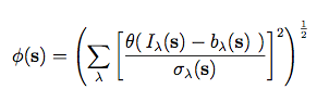
(Eq. 16)
2. Effects of confusion
3. Dealing with bright saturated stars
Last update: 2011 July 5
Previous page Next page
Return to Explanatory Supplement TOC