
| A Comparison of Responsivity Estimation Methodologies | |
Below we summarize our results of estimating the relative responsivity (flat-field calibration) from a recent 30 orbit simulation provided by N. Wright. Two estimation methods were explored:
Another concern is the presence latent-sources contaminating the responsivity maps. These are actually seen in the w3 and w4 maps (see Figures 3 and 4 - challenge yourself to find them!). If these are ~constant and persist for the duration over which a particular flat is created/applied, then these artifacts should divide out.
This is defined as the median of 100*(σf / f) over all pixels
where σf is the 1-sigma uncertainty in the resposivity
estimate f for a pixel.
This quantity is shown as a function of the number of input scans.
Note that 1 scan ~ 250 frames, so 8 scans ~ 2000 frames.
Table 1 shows results for
for the gradient method and Table 2 for the stacking method.
| Band | 1 scan | 2 scans | 3 scans | 4 scans | 5 scans | 6 scans | 7 scans | 8 scans |
|---|---|---|---|---|---|---|---|---|
| 1 | 11.407 | 6.892 | 5.895 | 4.870 | 4.479 | 3.976 | 3.755 | 3.443 |
| 2 | 4.582 | 2.787 | 2.380 | 1.970 | 1.809 | 1.608 | 1.517 | 1.392 |
| 3 | 0.385 | 0.261 | 0.216 | 0.184 | 0.166 | 0.150 | 0.140 | 0.130 |
| 4 | 0.392 | 0.270 | 0.222 | 0.190 | 0.171 | 0.155 | 0.144 | 0.134 |
| Band | 1 scan | 2 scans | 3 scans | 4 scans | 5 scans | 6 scans | 7 scans | 8 scans |
|---|---|---|---|---|---|---|---|---|
| 1 | 2.908 | 2.131 | 1.719 | 1.506 | 1.337 | 1.228 | 1.132 | 1.063 |
| 2 | 0.763 | 0.549 | 0.445 | 0.388 | 0.345 | 0.316 | 0.292 | 0.274 |
| 3 | 0.098 | 0.070 | 0.057 | 0.049 | 0.044 | 0.040 | 0.037 | 0.035 |
| 4 | 0.115 | 0.083 | 0.067 | 0.058 | 0.052 | 0.048 | 0.044 | 0.041 |
This is defined as the median absolute difference with respect to "truth":
100*median(|fest -
ftrue| / ftrue),
where fest is the estimated (measured)
responsivity for a pixel and
ftrue is the true value from the flat-field
used for the simulation. The median is over all pixels in the flat-field.
This quantity is shown as a function of the number of input scans.
Note that 1 scan ~ 250 frames, so 8 scans ~ 2000 frames.
Table 3 shows results for
for the gradient method and Table 4 for the stacking method.
| Band | 1 scan | 2 scans | 3 scans | 4 scans | 5 scans | 6 scans | 7 scans | 8 scans |
|---|---|---|---|---|---|---|---|---|
| 1 | 13.754 | 10.887 | 10.370 | 10.300 | 10.178 | 10.254 | 10.174 | 10.238 |
| 2 | 3.361 | 1.993 | 1.701 | 1.412 | 1.292 | 1.157 | 1.084 | 1.001 |
| 3 | 0.287 | 0.199 | 0.167 | 0.142 | 0.131 | 0.117 | 0.111 | 0.103 |
| 4 | 0.285 | 0.212 | 0.175 | 0.156 | 0.141 | 0.131 | 0.122 | 0.115 |
| Band | 1 scan | 2 scans | 3 scans | 4 scans | 5 scans | 6 scans | 7 scans | 8 scans |
|---|---|---|---|---|---|---|---|---|
| 1 | 2.294 | 1.758 | 1.475 | 1.340 | 1.233 | 1.172 | 1.112 | 1.076 |
| 2 | 0.565 | 0.420 | 0.351 | 0.314 | 0.286 | 0.269 | 0.254 | 0.243 |
| 3 | 0.068 | 0.049 | 0.040 | 0.035 | 0.032 | 0.029 | 0.027 | 0.026 |
| 4 | 0.081 | 0.058 | 0.048 | 0.042 | 0.038 | 0.035 | 0.032 | 0.031 |
All assume 2-scans worth of frames (1 orbit or ~ 500 frames).
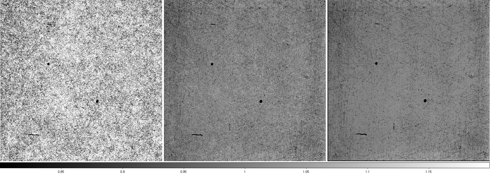 |
| Figure 1 - Band 1: From left to right: Flat estimated from gradient method; from stacking method; and truth used in simulation. Click to enlarge. |
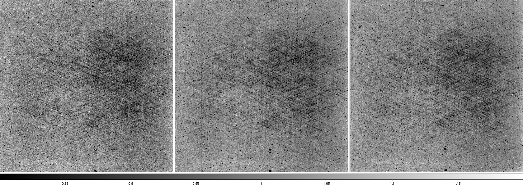 |
| Figure 2 - Band 2: From left to right: Flat estimated from gradient method; from stacking method; and truth used in simulation. Click to enlarge. |
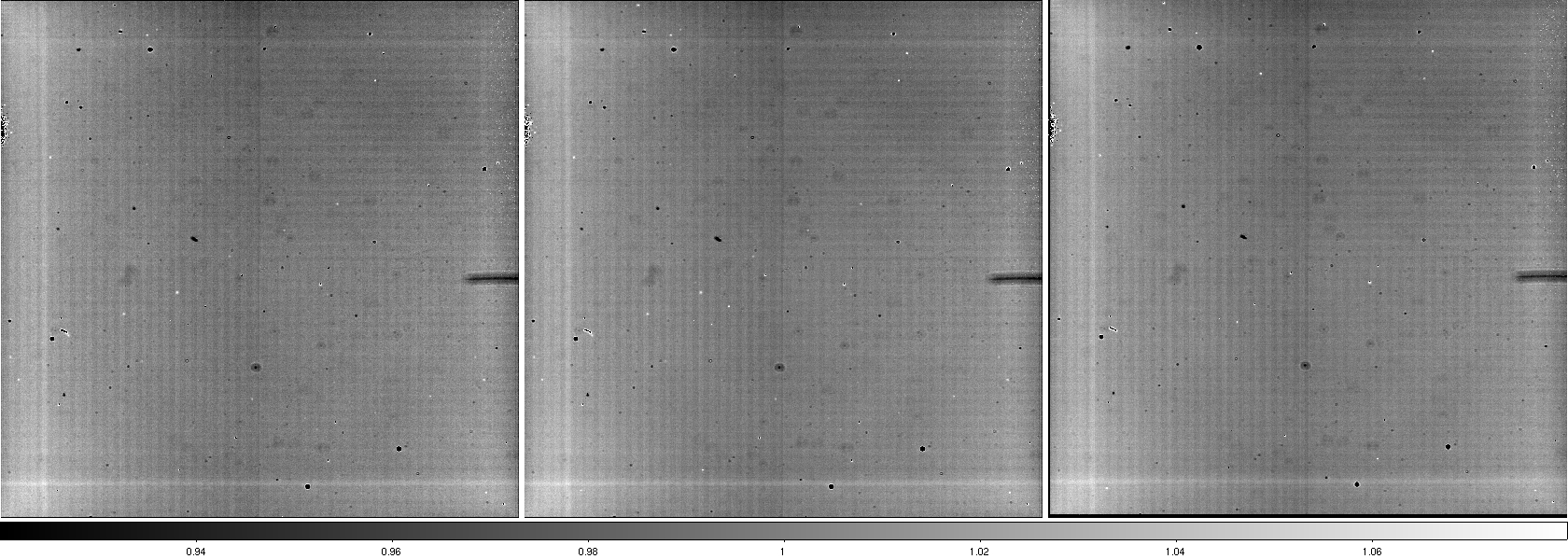 |
| Figure 3 - Band 3: From left to right: Flat estimated from gradient method; from stacking method; and truth used in simulation. Click to enlarge. |
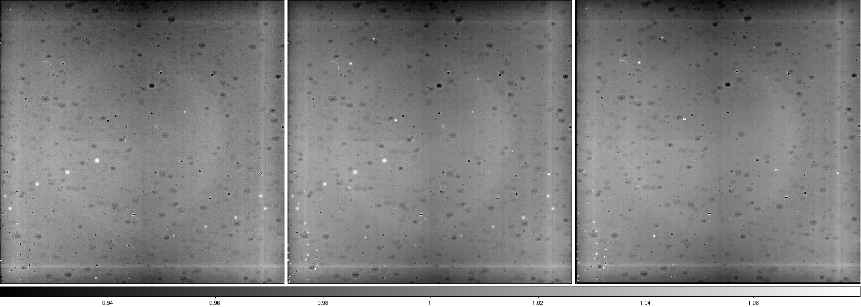 |
| Figure 4 - Band 4: From left to right: Flat estimated from gradient method; from stacking method; and truth used in simulation. Click to enlarge. |
 |
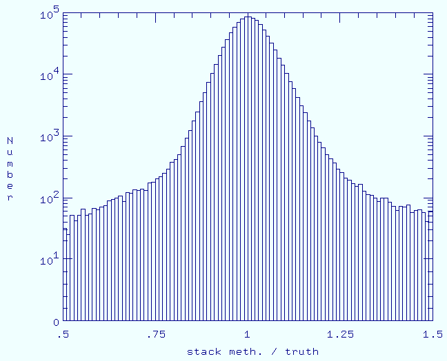 |
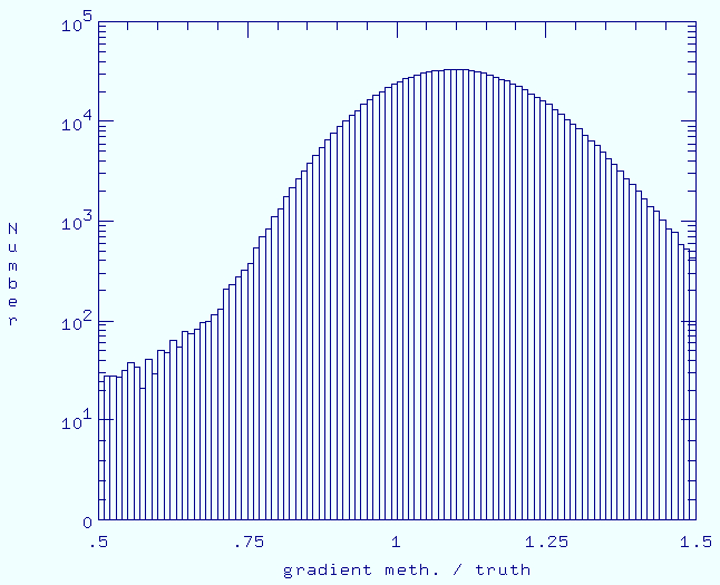
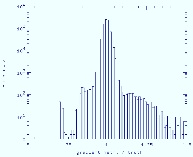
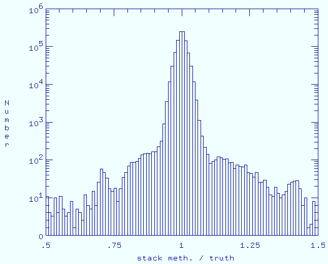
| Gradient method / Truth | Stacking method / Truth |
| Figure 5 - Band 1 histograms of ratio of estimated to true responsivity map for each method. Click any panel to enlarge. | |
 |
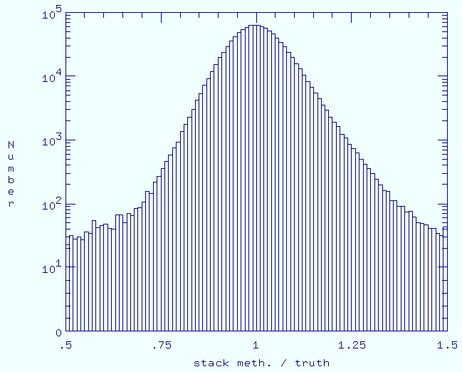 |
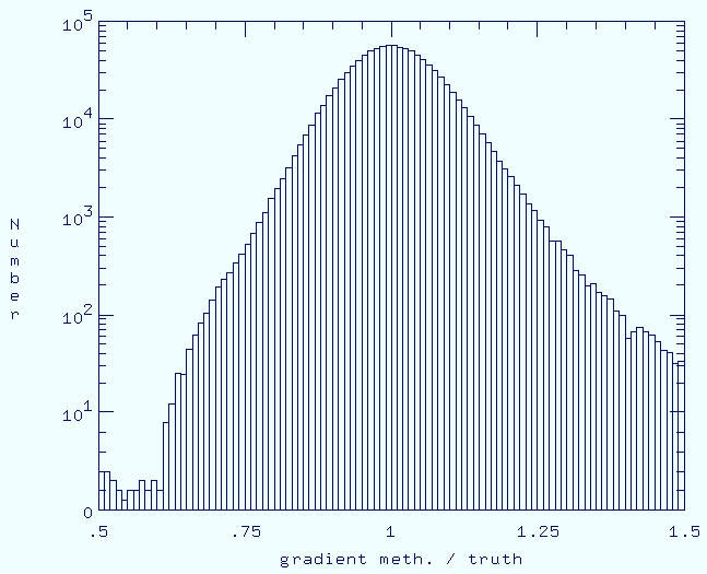
| Gradient method / Truth | Stacking method / Truth |
| Figure 6 - Band 2 histograms of ratio of estimated to true responsivity map for each method. Click any panel to enlarge. | |
 |
 |
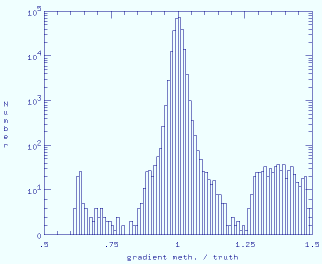
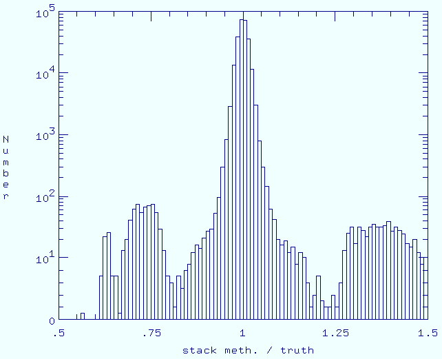
| Gradient method / Truth | Stacking method / Truth |
| Figure 7 - Band 3 histograms of ratio of estimated to true responsivity map for each method. Click any panel to enlarge. | |
 |
 |
| Gradient method / Truth | Stacking method / Truth |
| Figure 8 - Band 4 histograms of ratio of estimated to true responsivity map for each method. Click any panel to enlarge. | |