


In this section we describe the depth-of-coverage of the AllWISE Data Release area and explain some of the issues with the pathologies of low coverage areas. For the purposes of this section, the term "Sky Coverage" refers generically to the topic of the WISE dataset spatial surveying features; when appropriate, the term "depth-of-coverage" is used to refer specifically to the number of observations at a specific point on the celestial sphere, and the term "Catalog source density" is used to refer to the number density of Catalog sources extracted in a small region.
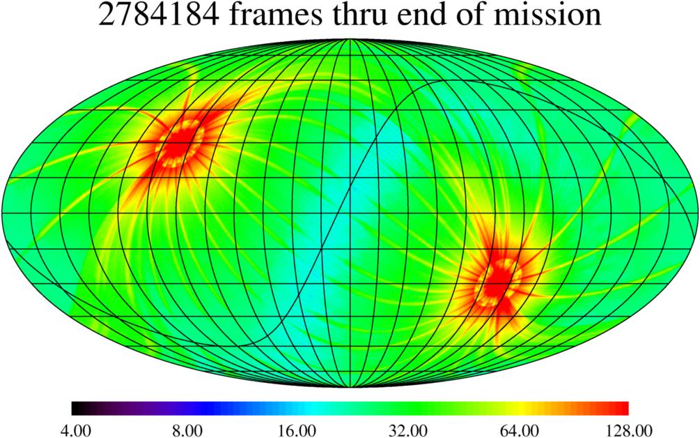
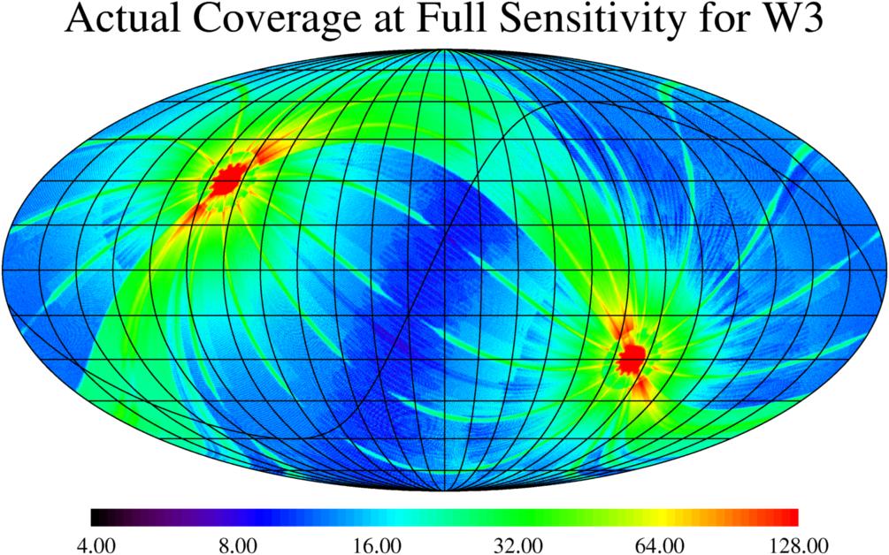
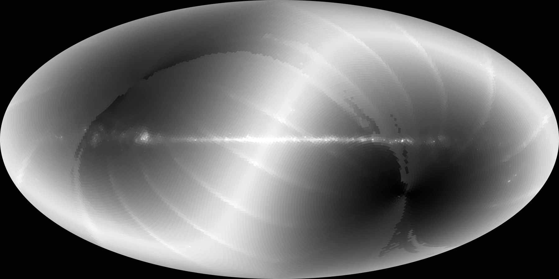
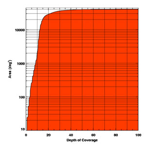
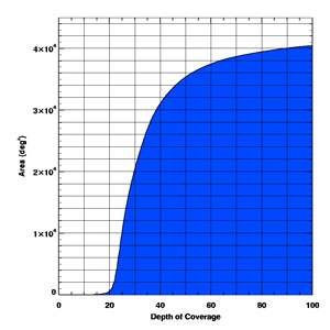
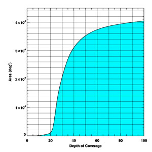
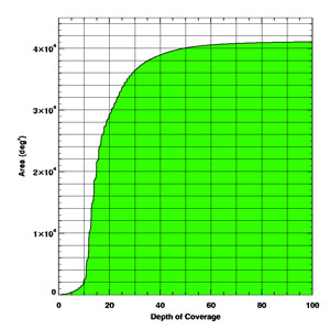
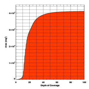
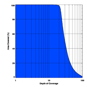
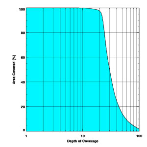
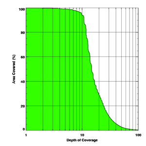
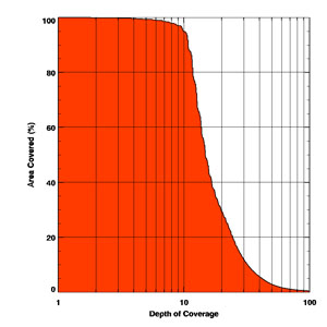
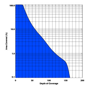
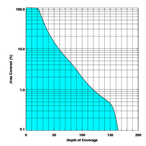
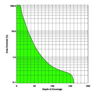
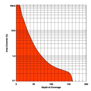
The WISE survey strategy was designed to provide at least 8 frames of coverage on at least 99% of the sky in the 6-month minimum all-sky survey interval. This minimum coverage was required in order to achieve sensitivity limits, and allows for coverages lost due to proximity to the Moon and the SAA, and further would have accommodated a recovery period in the event of any satellite anomaly (although no such anomalies caused the loss of any data). As a result, the expected whole-mission data downlink produce an ab initio depth-of-coverage as shown in Figure 1; the cryogenic portion of the mission produces the coverage shown in Figure 2 for bands W1 and W2. Because of the gradual degradation of performance at cryogen loss, the depths-of-coverage of W3 and W4 vary slightly from that shown in Figure 2; these are shown in Figure 3 and Figure 4.
 |
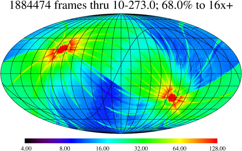 |
| Figure 1 - During the entire WISE operations period, covering more than a year, a total of 2,784,184 framesets were taken and downloaded. The depth of coverage across the whole sky in Galactic coordinates shows the buildup near the ecliptic poles. | Figure 2 - The cryogenic portion of the mission, those framesets which will be included in the Final Data Release, lasted until cryogen depletion in October 2010. Up to that time, all W1 and W2 data cover the sky at a depth of more than 8 using 18,844,474 framesets. |
 |
 |
| Figure 3 - As WISE approached cryogen loss, the telescope began to warm up. W3 integration times were reduced to prevent saturation once the telescope had reached 45 K. The actual coverage at full integration time is somewhat shallower for W1 and W2. | Figure 4 - As WISE approached cryogen loss, the telescope began to warm up and the W4 detectors saturated. The actual a priori coverage at 22 microns is therefore shallowest of all the WISE bands. Even so, the usable survey coverage allowed 97.9% of the sky to be seen 8 times or more. |
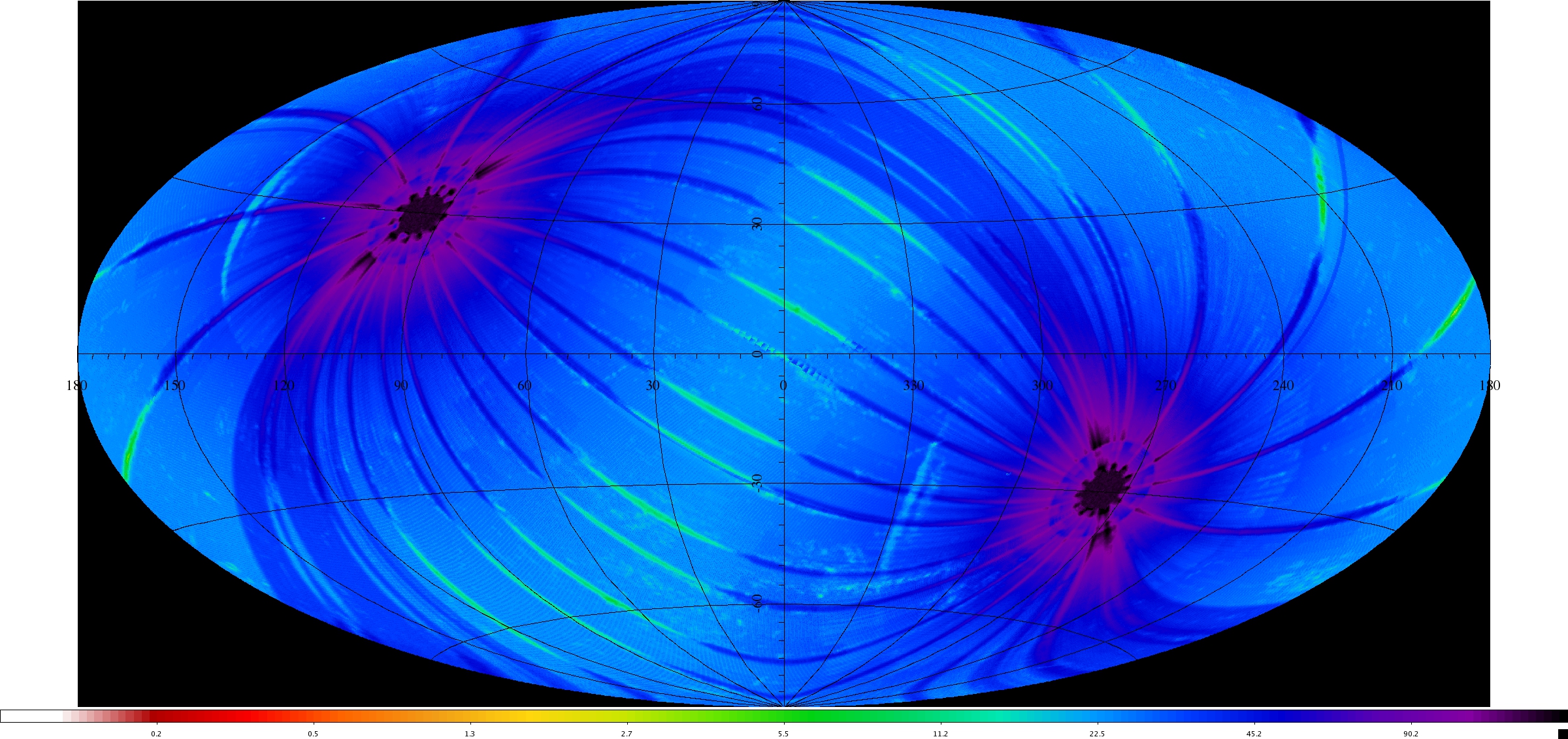
WISE imaged the entire sky with multiple, independent exposures in all four bands obtained simultaneously for the duration of its full cryogenic survey. The AllWISE Data Release includes data taken from 7 January 2010 to 1 February 2011, processed with improved calibrations and reduction algorithms as compared to the All-Sky Data Release. WISE completed its first all-sky coverage on 17 July 2010 and surveyed an additional 20% of the sky before the onset of cryogen depletion. A further 30% of the sky was conducted during telescope warmup, during which W4 was inactive and W3 continued to take data a decreasing sensitivity. Following full cryogen depletion, an additional 70% of the sky was surveyed in only W1 and W2 up to the completion of mission operations. Because of WISE's survey scanning strategy, the depth of coverage ranges from 11.9 exposures of each point on the ecliptic plane in W3 and W4 (23.5 in W1/W2), increasing to over 3000 exposures at the ecliptic poles (see Figure 5 and Figure 6).
The AllWISE Data Release area is comprised of 18,240 Atlas Tiles, each Tile spanning 1.564° × 1.564° in 4095 × 4095 pixels at a resolution of 1.375″ per pixel. These Tiles are delivered in FITS format image sets, consisting of an intensity image, the corresponding uncertainty image, and a depth-of-coverage map at each of the four WISE bands. The celestial sphere is tessellated with the grid of 18,240 such Tiles on an equatorial projection for the purpose of combining the WISE single-exposure images and extracting final source information. The Tiles are distributed in 119 iso-declination bands with 238 Tiles on the celestial equator decreasing to six Tiles in the |δ|=89.35° declination band. Tiles are designed to overlap by 180″ in RA and Dec on the equator, increasing in RA overlap towards the equatorial poles. This overlap means that the total image content of the tiles corresponds to 44,620.357 deg2, or roughly 108.163% of the sky. The extra 8.163% represents the overlap regions, but for the purpose of quantifying the sky coverage below we have renormalized to 100% of the celestial sphere of 41,252.961 deg2.
 |
|
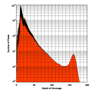
| Figure 5 - Ecliptic Hammer-Aitoff projection sky map showing the area covered by the AllWISE Data Release; the survey scan pattern is most evident in this projection. The colors encode the average number of single 7.7/8.8 sec WISE exposure frames covering 15´ × 15´ bins. The legend on the bottom gives the frame coverage depth. | Figure 6 - Differential area as a function of average frame depth-of-coverage in the AllWISE Data Release, computed in 15´ × 15´ bins. The peak at ≈22 is the 'typical' two-epoch coverage; the secondary peak at ≈36 is the coverage for the ≈10% of the sky that was seen a third time; the peak at ≈160 is the constant-viewing area near the Ecliptic poles. |
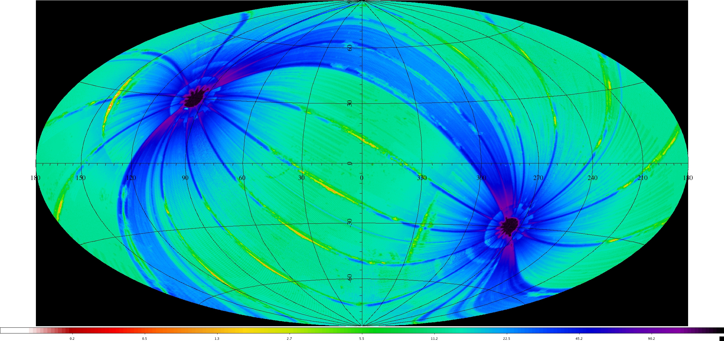
The post facto coverage is shown in Figure 7, computed in 15´ × 15´ bins and shown in Galactic coordinates in order to match the images following.
 |
 |
| W1 | W2 |
 |
 |
| W3 | W4 |
| Figure 7 - Hamer-Aitoff equal-area projection of the AllWISE Data Release depth of coverage in each band in Galactic coordinates. | |
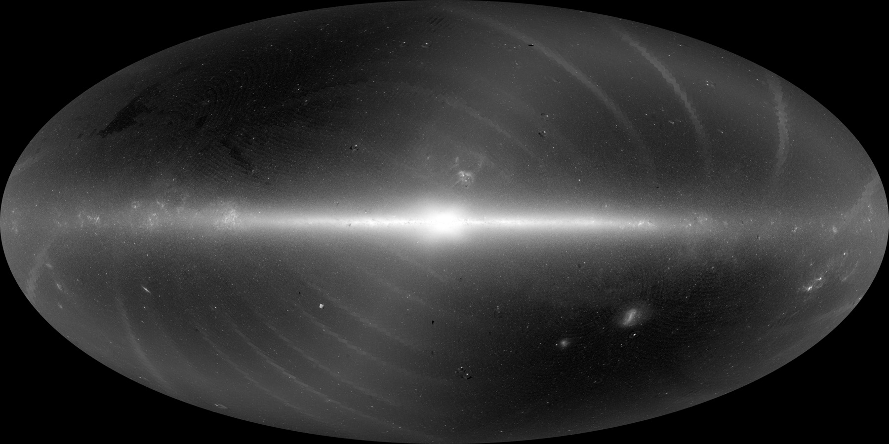
Below in Figures 8 and 9 are full-sky Hammer-Aitoff equal-area projection images of the AllWISE Data Release Atlas Tiles oriented in Galactic coordinates. The slight differences in coverage at the four wavelengths can be seen, as can the strips of enhanced background due to the proximity of the Moon (seen as segments running slightly clockwise of vertical). The plane of the galaxy runs prominently throughout, as does a diffuse zodiacal light component. Those with sharp eyes will be able to discern banding in the zodiacal light running along Ecliptic longitude.
 |
| Figure 8 - Hammer-Aitoff equal-area projection of the AllWISE Data Release intensity images at 12′ resolution, manufactured by direct addition of the 44,620.357 deg2 in all 18,240 Atlas Tiles. A large (35.2MB) version of this image at 1.5′ resolution is available for download. This and the following images are in Galactic coordinates centered on the Galactic center; the plane of the Milky Way runs horizontally. The Ecliptic can be seen as the gold-toned swath running across the center, with strips of elevated background due to residual Moon glow visible as white bars perpendicular to the Ecliptic. |
 |
 |
| W1 | W2 |
 |
 |
| W4 | W4 |
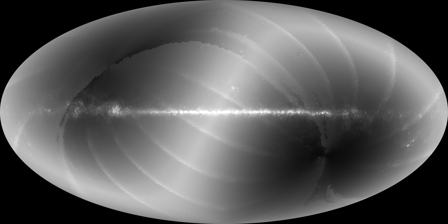
| Figure 9 - Hamer-Aitoff equal-area projection of the AllWISE Data Release intensity images in each band. | |
The AllWISE survey depth-of-coverage varies across the sky because of the survey scanning strategy, as described in Section III.4 of the WISE All-Sky Release Explanatory Supplement. There are typically at least 12 independent exposure frames contributing to each point on the sky near the ecliptic plane. The depth increases towards the ecliptic poles, reaching a maximum of ~160 frames at the highest ecliptic latitudes in the AllWISE Data Release (Figure 5). Visible in Figure 5 are some small patches with decreases in frame coverage caused by filtering out exposures considered to be of lower quality because of contamination by scattered moonlight (within 20° of the ecliptic), image quality degradation due to flight system motion, or other events. Pixel-level frame coverage information is provided in the WISE Atlas Tile Depth-of-Coverage Maps. Here we present ensemble statistics of the coverage achieved for this data release.
Each Atlas FITS image contains in the header some high-level quantification of the depth-of-coverage for that Tile. This information may also be accessed in the Atlas Inventory metadata table. (Full depth-of-coverage information can readily be derived from the Atlas Depth-of-Coverage maps, for those who wish to determine this on a per-pixel level). The header keywords are listed in Table 1.
| Keyword | Meaning | Data Type |
|---|---|---|
| MEDCOV | Median depth-of-coverage | float |
| MINCOV | Minimum depth-of-coverage | float |
| MAXCOV | Maximum depth-of-coverage | float |
| LOWCOVPC | Percent of pixels with depth ≤4¥ | float |
| LOWCOPC | Percent of pixels with depth ≤6† | float |
| NOMCOVPC | Percent of pixels with depth ≤8‡ | float |
Notes:
¥ Coverage of 4 was the metric used as the WISE mission's
Level 1 requirements for sky coverage, specifically that at least 95% of the
sky should be covered to this depth or greater.
† Coverage ≤5 implies pixels that are at or below the
threshold for statistically viable outlier detection and rejection
(see below), and so can be contaminated by random
pixel variations such as cosmic rays.
‡ Coverage ≤8 implies regions where the coverage is less
than the nominal coverage required for the desired minimum sensitivity
goals.
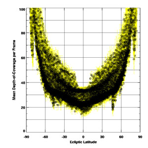
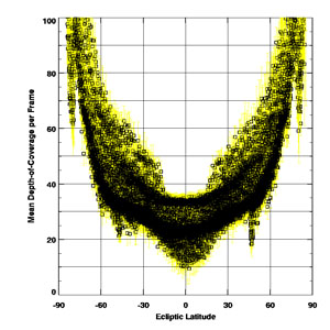
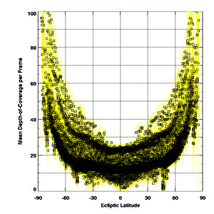
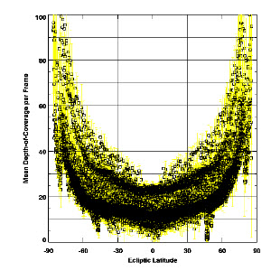
The median depth-of-coverage across the full AllWISE Data Release is 30.171±0.023 in W1, 29.998±0.032 in W2, 14.858±0.002 in W3, and 14.861±0.003 in W4. (The reason for the uncertainty is that the median is determined by fitting to a histogram of the 305,867,016,000 image pixels per band, a process that necessarily results in some imprecision.) In Figures 10-16 below, we show more complete statistics of the depth-of-coverage distributions in this data release.
 |
 |
| W1 | W2 |
 |
 |
| W3 | W4 |
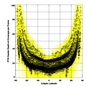
| Figure 10 - Calculated pixel-level depth-of-coverage vs. ecliptic latitude for each band, plotted on a per-Tile basis; the yellow region indicates the dispersion of the distribution in each Tile, calculated via an outlier-resistant variance estimator. The typical Tile coverage can be seen as the heavy convex band; the doubling of coverage in W1/W2 versus W3/W4, and a 3:2 ratio in certain areas, is visible. Higher coverage near the Ecliptic poles is clipped for clarity. | |
 |
 |
| W1 | W2 |
 |
 |
| W3 | W4 |
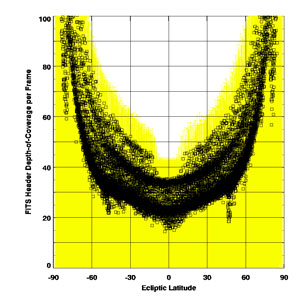
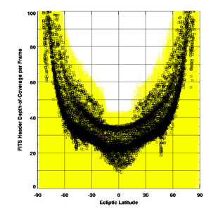
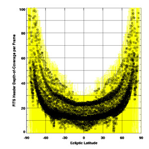
| Figure 11 - FITS header values of the median coverage (MEDCOV) in each band vs. ecliptic latitude; the yellow region indicates the minimum (MINCOV) and maximum (MAXCOV) coverage in each Tile. | |
 |
 |
| W1 | W2 |
 |
 |
| W3 | W4 |
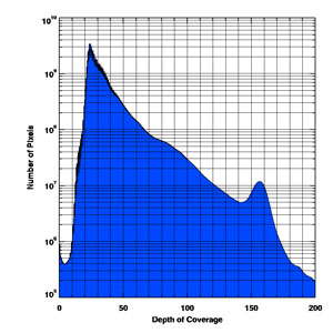
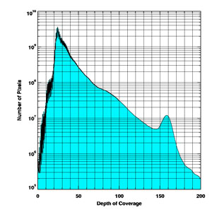
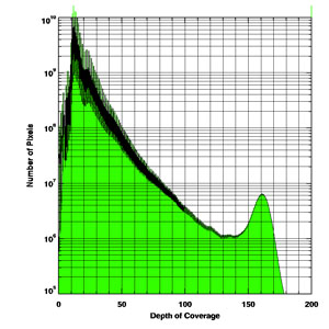
| Figure 12 - Histogram of per-pixel depth-of-coverage in each Tile for each band for the entire AllWISE Data Release. The doubling of coverage in W1/W2 can be see in the peak position of the histograms. Note that this is summed over Tiles, and so there is a slight overlap resulting in a double-counting of certain spatial pixels on the sky as described above. The bin width is in units of 1/8th of a coverage, which can be non-integral (see section II.3.d of the WISE All-Sky Release Explanatory Supplement). | |
 |
 |
| W1 | W2 |
 |
 |
| W3 | W4 |
| Figure 13 - Cumulative histogram of the area in square degrees resulting from integrating the curves in Figure 12, above. | |
 |
 |
| W1 | W2 |
 |
 |
| W3 | W4 |
| Figure 14 - Same as Figure 13, but in a linear scale. | |
 |
 |
| W1 | W2 |
 |
 |
| W3 | W4 |
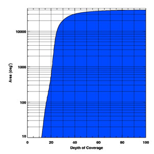
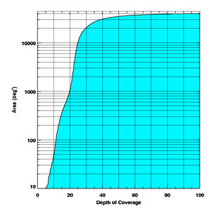
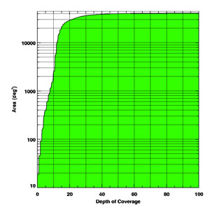
| Figure 15 - The ordinate shows the percentage of the sky covered in the AllWISE Data Release Tiles to a depth of at least that indicated on the abscissa, for each band. | |
 |
 |
| W1 | W2 |
 |
 |
| W3 | W4 |
| Figure 16 - Same as Figure 15, but in log-linear scale to highlight the small area covered to high depth. | |
Here we provide statistics calculated across the AllWISE Atlas Tiles on a per-pixel basis. Table 2 lists the pixel-level depth of coverage for each WISE band as a function of fraction of sky covered. For example, in band W3 (12 microns), 50% of the sky has been covered at a depth of ≥14.86; in band W2 (4.6 microns), 1% of the sky has been covered at a depth of ≥119.55.
Table 2 - Depth of coverage for each WISE band as a function of
fraction of sky covered. For example, in band W1 (3.4 microns),
50%
of the sky has been covered at a depth of ≥30.17; in band W3 (12
microns), 95% of the sky has been covered at a depth of ≥9.81.
| Band | W1 | W2 | W3 | W4 |
| 99.9% | ≥14.31 | ≥9.61 | ≥0.99 | ≥1.87 |
| 99.5% | ≥17.80 | ≥12.95 | ≥3.74 | ≥4.35 |
| 98% | ≥20.55 | ≥19.07 | ≥6.94 | ≥7.85 |
| 95% | ≥21.84 | ≥21.46 | ≥9.81 | ≥9.97 |
| 90% | ≥22.84 | ≥22.65 | ≥10.83 | ≥10.83 |
| 75% | ≥25.06 | ≥24.93 | ≥12.27 | ≥12.45 |
| 50% | ≥30.17 | ≥30.00 | ≥14.86 | ≥14.86 |
| 25% | ≥39.85 | ≥39.78 | ≥21.90 | ≥22.11 |
| 10% | ≥57.88 | ≥58.24 | ≥31.86 | ≥31.98 |
| 5% | ≥84.24 | ≥77.72 | ≥41.83 | ≥41.87 |
| 1.0% | ≥118.77 | ≥119.55 | ≥71.82 | ≥71.89 |
| 0.5% | ≥145.87 | ≥146.96 | ≥93.53 | ≥93.58 |
| 0.2% | ≥158.56 | ≥160.01 | ≥153.62 | ≥153.91 |
As can be seen below in Table 3, there are several square degree areas — a small percentage of the sky, but not negligible — where the coverage is zero. While WISE imaged every point on the sky multiple times during the full cryogenic mission, not every Single-exposure image was of sufficient quality to incorporate in the Multiframe Pipeline processing (cf. V.1.b). Because of the many factors that impact the usable depth-of-coverage, these are regions within the footprints of the 18,240 Atlas Tiles that cover the full sky for which the effective depth-of-coverage is very low or even zero. If there is insufficient coverage in these regions, the corresponding pixels in the Atlas Images may have "NaN" values, and no sources can be detected in those locations. We provide Table 3 to illustrate the scope of the low coverage regions in the Atlas Tiles. The most important rows are those that show the fraction of sky the is not covered at all (COV=0) or covered at a low enough level that outlier rejection is invalidated (COV<5), hence detection reliability will be significantly impacted.
Consequently, although WISE observed every point on the sky multiple times, there may be insufficient usable Single-exposure data to have corresponding Atlas Image or Source Catalog data. Viewing the Atlas Depth-of-Coverage maps is the best way to determine if a region of interest to you may have reduced coverage, and therefore lower sensitivity, and/or missing detections in the Source Catalog.
All of Single-exposure images, regardless of quality, are available in the All-Sky Release, 3-Band Cryo Release, and Post-Cryo Release. Therefore, you may find image and extracted source information in those archives for regions with low and/or no coverage in the AllWISE Release Atlas and Source Catalog.
| Band | W1 | W2 | W3 | W4 |
| COV=0 | 0.0005% | 0.0005% | 0.044% | 0.022% |
| 0.22°² | 0.19°² | 18.211°² | 9.031°² | |
| COV<4 | 0.005% | 0.009% | 0.616% | 0.380% |
| 2.24°² | 3.55°² | 254.13°² | 156.88°² | |
| COV<5 | 0.006% | 0.016% | 0.963% | 0.625% |
| 2.67°² | 6.76°² | 397.46°² | 257.90°² | |
| COV≥8 | 99.990% | 99.939% | 97.251% | 97.883% |
| 41,249°² | 41,228°² | 40,119°² | 40,380°² | |
| COV≥12 | 99.974% | 99.659% | 75.731% | 77.450% |
| 41,242°² | 41,112°² | 31,241°² | 31,950°² |
The median depth-of-coverage can be calculated for portions of the sky to highlight the effect of spatial selections. In each of Ecliptic, Galactic, and Equatorial coordinates, Table 4 shows the median depth-of-coverage for W1 as a function of latitude cuts. In this case, the pixel-level median is calculated on a per-Tile basis and the Tile central latitude is used; hence, there is some inaccuracy in the highest latitude cuts where the depth-of-coverage changes rapidly with latitude on scales smaller than a Tile (1.564°). The depth-of-coverage for W2 is similar; for W3 and W4, the depth-of-coverage is similar to that yielded in the All-Sky Release, available in Table 4 of section VI.2.b.i in the WISE All-Sky Release Explanatory Supplement.
| Latitude Cut | ECL | GAL | EQU |
| |lat|≥ 5° | 31.6 | 30.8 | 31.5 |
| |lat|≥10° | 32.1 | 30.8 | 31.9 |
| |lat|≥15° | 32.9 | 30.7 | 32.4 |
| |lat|≥20° | 34.0 | 30.7 | 33.4 |
| |lat|≥25° | 35.6 | 30.8 | 34.5 |
| |lat|≥30° | 37.9 | 30.8 | 36.2 |
| |lat|≥40° | 43.3 | 31.0 | 40.6 |
| |lat|≥50° | 52.9 | 31.0 | 45.8 |
| |lat|≥60° | 65.2 | 30.6 | 49.0 |
| |lat|≥70° | 85.4 | 29.7 | 52.8 |
| |lat|≥80° | 98.4 | 29.0 | 55.4 |
| |lat|≥85° | 149.3 | 29.0 | 55.5 |
| |lat|≥89° | 157.1 | 28.1 | 56.5 |
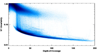
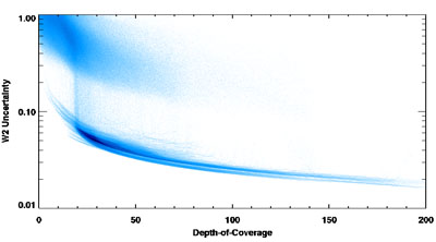
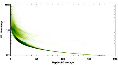
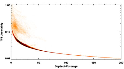
It is expected that, since depth of coverage is linearly related to the amount of time spent collecting photons from each position on the sky, the sensitivity should improve approximately as the square root of the depth of coverage. One of the Atlas products is the UNCertainty data in the same spatial format as the INTensity and COVerage data. A description of the uncertainty maps is found in section Section IV.1.a. The uncertainty map stores the 1-σ uncertainty per pixel corresponding to the co-added intensity values in the primary Atlas Image, in the same units of DN (cf. section IV.1.a on the use of uncertainty maps in aperture photometry). These uncertainty maps are based solely on prior knowledge of the instrument response (as opposed to a posteriori data-derived estimates), and hence do not include any component of confusion noise, which may be significant in regions with high source density and/or complex background emission.
Figure 17 shows a plot of the per-pixel uncertainty map in DN vs. the depth-of-coverage. Since each plot consists of all 305,867,016,000 pixels, the intensity has been logarithmically scaled better to highlight the scatter in the distribution. The lower boundary, which contains a large fraction of the total pixels in each band, shows that the uncertainty at pixel j scales very closely to σj ∝ 1/√Nj, where Nj is the depth-of-coverage at pixel j.
 |
 |
| W1 | W2 |
 |
 |
| W3 | W4 |
| Figure 17 - Uncertainty vs. depth of coverage evaluated on a per-pixel basis for each band. | |
The WISE scan strategy was designed to allow for repeat viewings of at least 8 times on every point on the sky, with accommodations allotted for planned survey motions and margins for unplanned survey interruptions. The achieved characteristic coverage is slightly higher than this because the survey was not interrupted. However, there are some regions that have anomalously low effective coverage in the Atlas Images and Source Catalog because some Single-exposure framesets were rejected from Multiframe processing due to poor assessed quality (i.e. see V.1.b). Some of the reasons for low coverage are summarized below. Others may be found in the All-Sky Release Explanatory Supplement - Section VI.2.c.
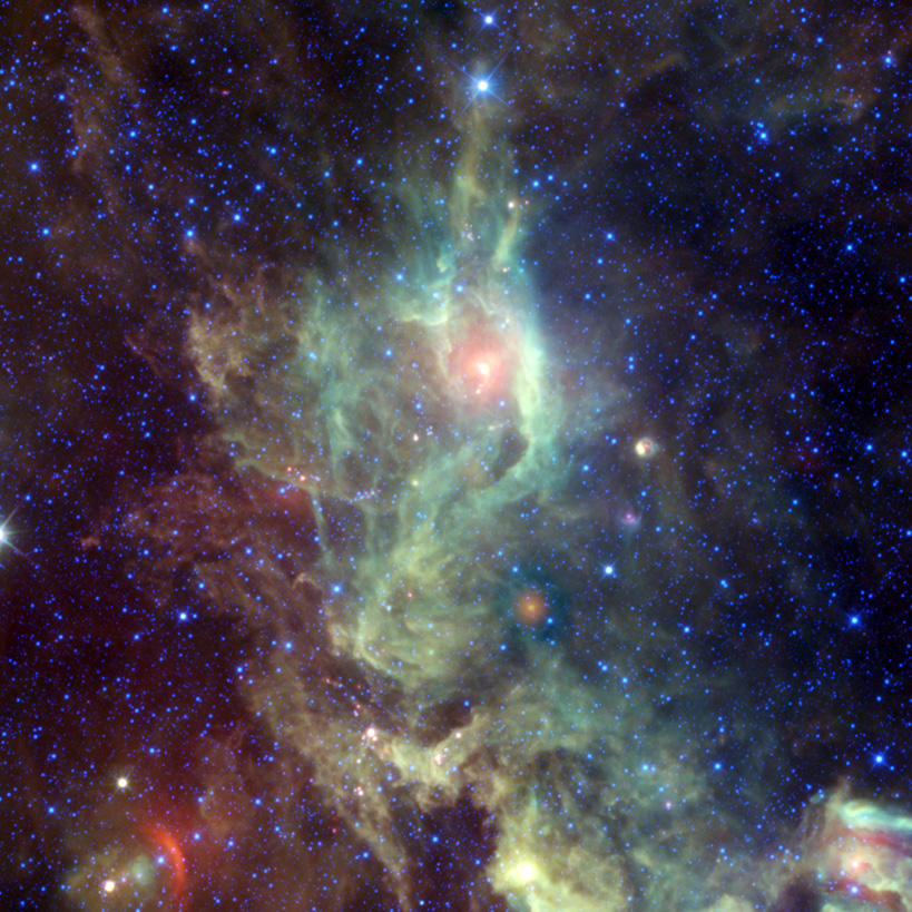
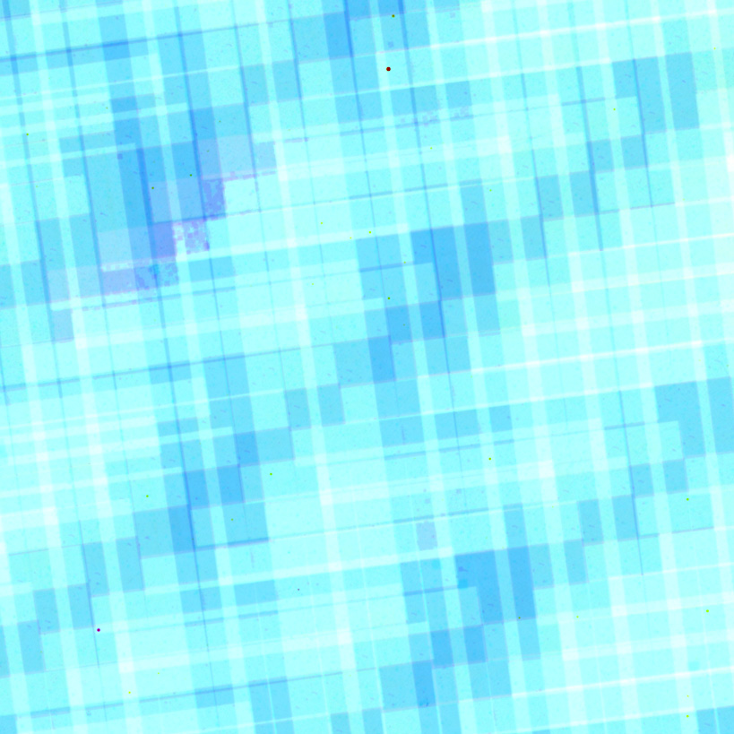
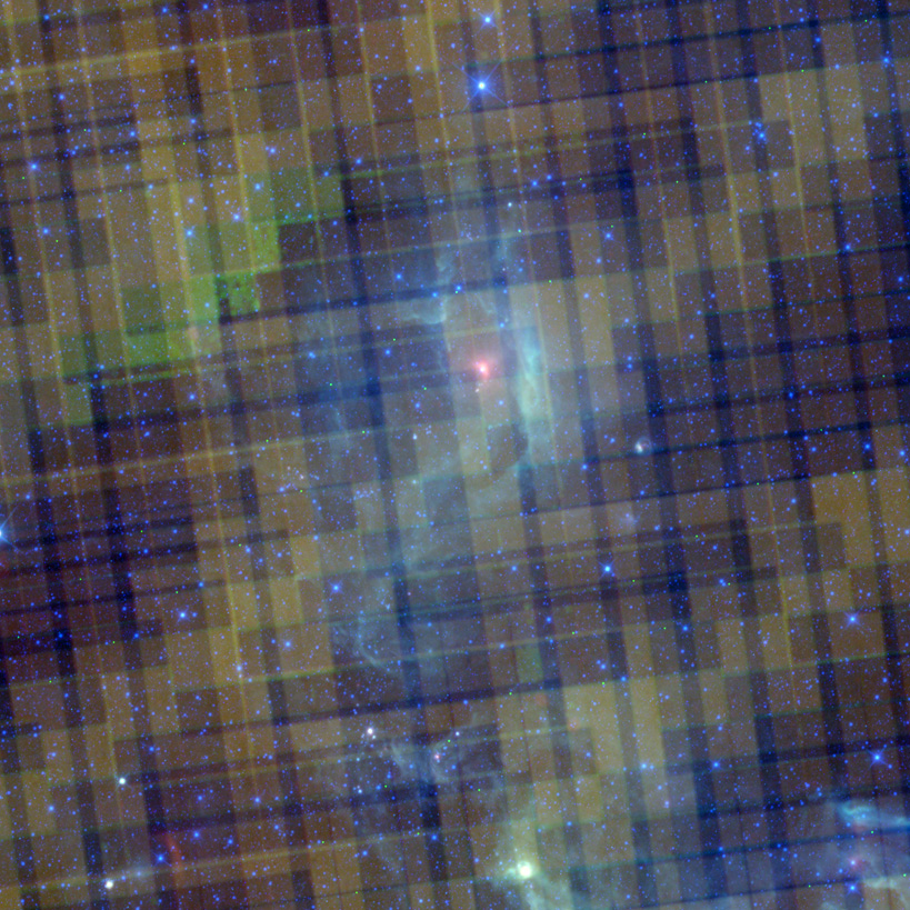
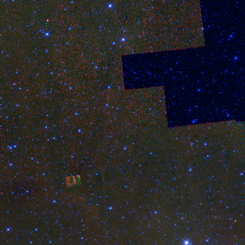
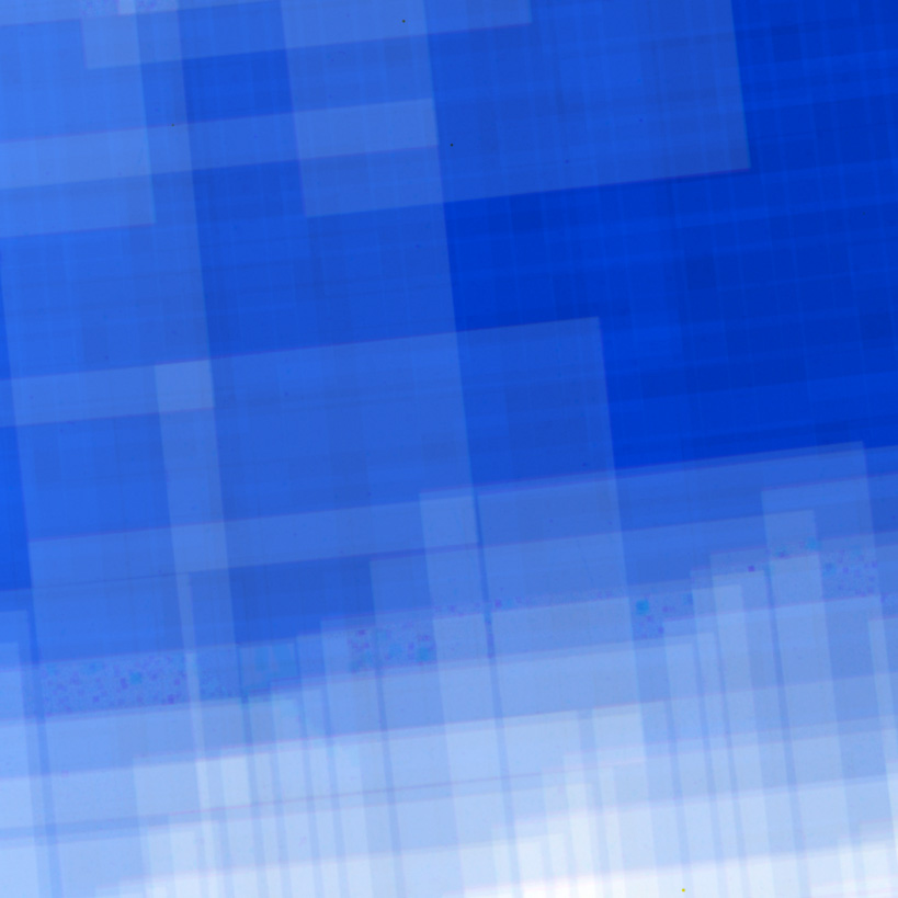
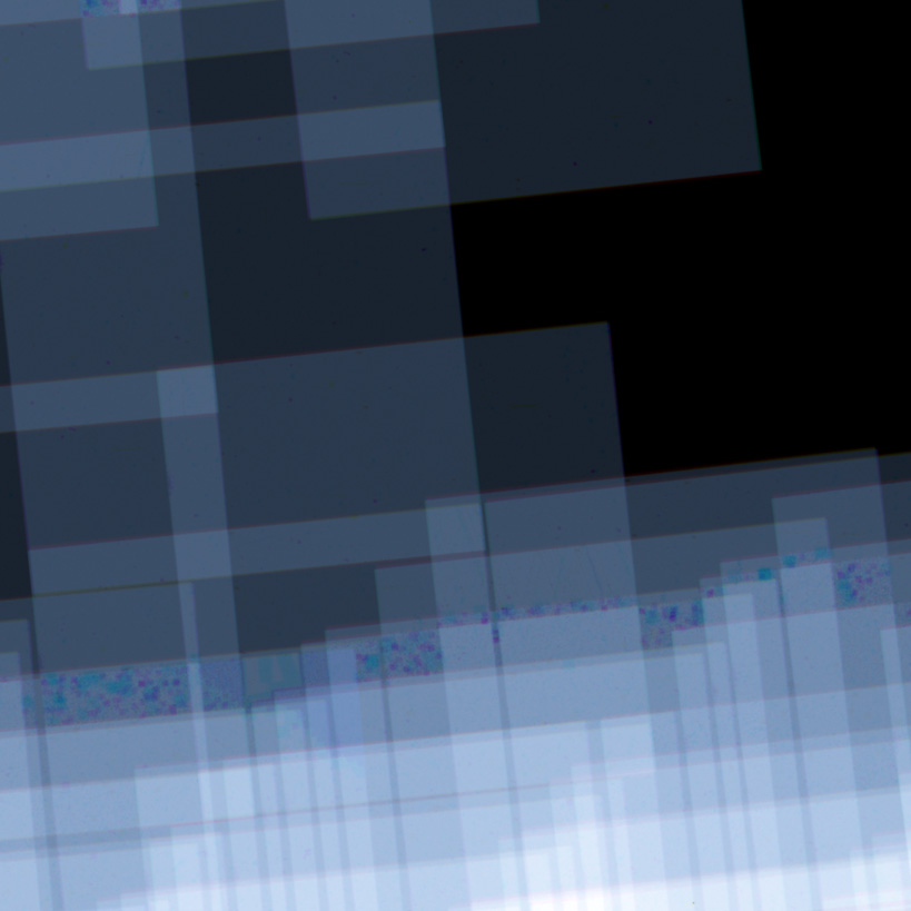
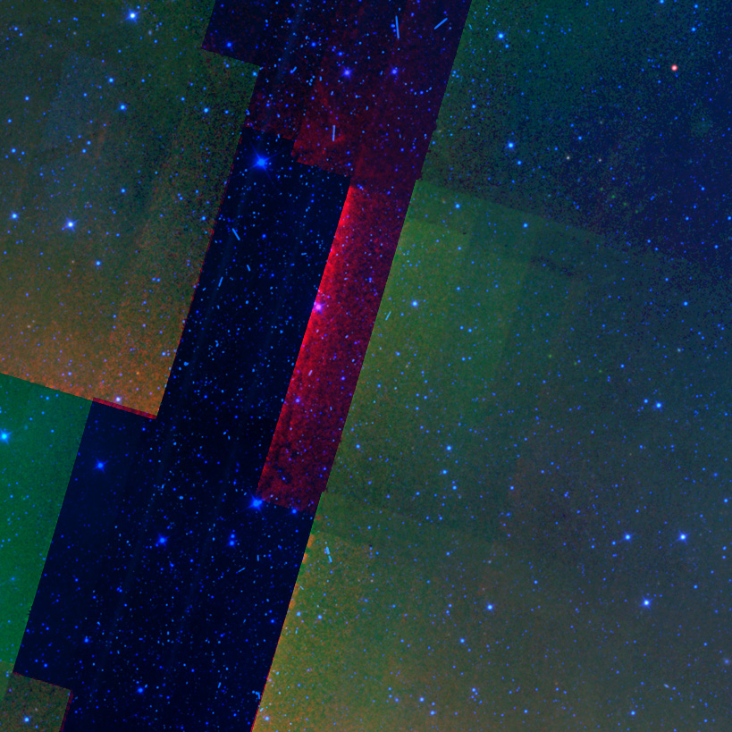
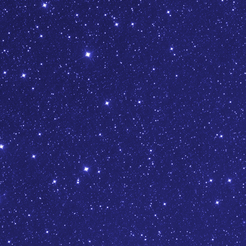
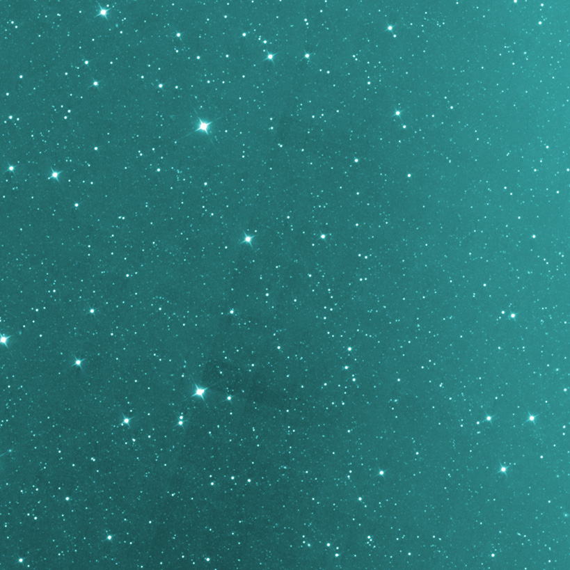
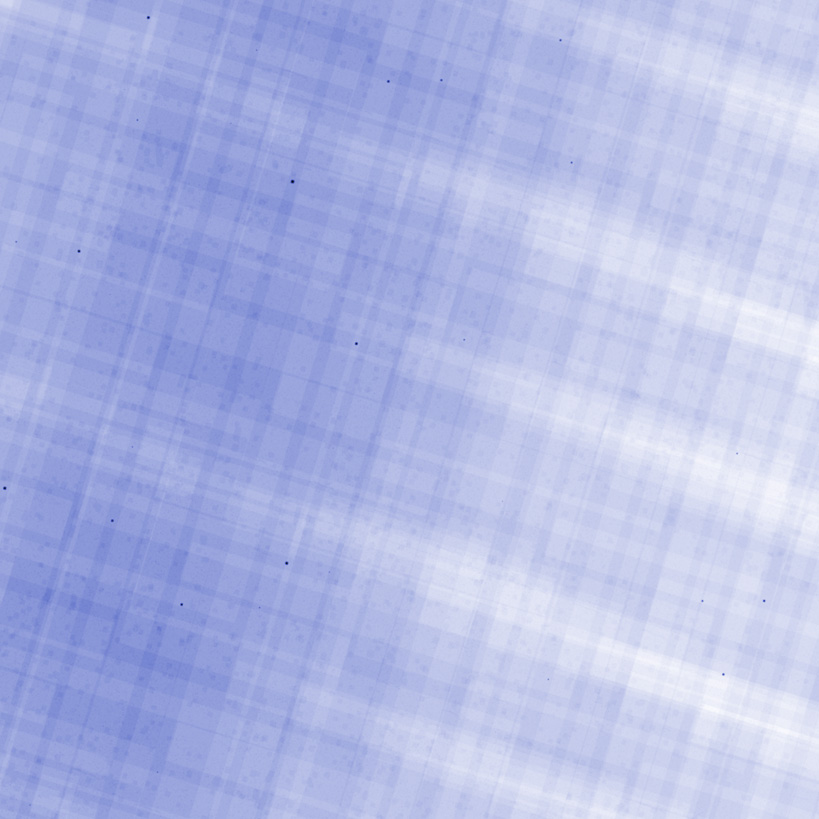
The AllWISE Data Release Atlas Tiles consist of three products per band: an INTensity image, a COVerage image, and an UNCertainty image. An example of these three products, combined into a 4-color image, is shown in Figure 18.
 |
 |
 |
| W1-4 INT | W1-4 COV | W1-4 UNC |
| Figure 18 - An image of 1061m107_ac51, a single AllWISE Atlas tile in the area of IC2177, the Seagull Nebula, showing the direct image, the depth of coverage of the image, and the uncertainty of the image. The depth of coverage shows its inverse effect on the uncertainty and hence implicitly on the significance of detection of sources in the direct image. Where there is lower coverage, there will be higher uncertainty and poorer source extraction will arise. | ||
Comparison of the achieved Atlas tile coverage (Figures 5, 7, 8, and 9) with the survey frame coverage (Figures 1-4) illustrates some loss of coverage, particularly in bands W3 and W4. Among the most significant are the horizontal bands at Ecliptic λ,β= 100°,+45° and 290°,-45° (Equatorial α, δ= 110°,+70° and 310°,-70°). Early in the survey, the spacecrafts' magnetic torque rods were enabled to dump accumulated momentum when scans approached within 45° of the ecliptic poles. Activating the torque rods resulted in a small jump in the telescope pointing and smearing of the resulting images. Because the smearing occurred near the same point on each orbit, and the smeared images were flagged as having degraded image quality in the QA process, low-coverage "holes" developed at those locations. Later in the survey (2010 May 02), torque rod enabling was staggered between 45, 57.5 and 70° latitude on alternating orbits so that any image smearing would not occur at the same point on the sky on each orbit. It was hoped that the WISE cryogenic mission would last long enough to enable a repeat visit of the affected areas, but some small portions of sky were never revisited and so the gaps remain in W3 and W4. A single Atlas Tile containing such a gap, 1004p696, is shown in Figure 19.
| AllWISE: |
 |
 |
| W1-4 INT | W1-4 COV | |
| All-Sky: |
 |
 |
| W1-4 INT | W1-4 COV | |
| Figure 19 - Intensity and coverage images of a single Atlas tile (1004p696) near (95,+45) Ecliptic, showing a clear gap in coverage where data are missing in both the AllWISE (top) and All-Sky (bottom) images. This gap spans across portions of several neighboring Tiles at one of the torque rod gashes. The coverage is very similar at W3 and W4 to the coverage in the earlier All-Sky Data Release wavelengths, since it was induced by a common-mode issue at the spacecraft level. However, the extended duration of the data in the AllWISE release allows W1 and W2 to re-view those regions (note the blue stars in the gap region in AllWISE, hence the coverage is adequate (although roughly half what it is in the surrounding non-gap area). | ||
When WISE observes near the moon, stray light can contaminate images significantly enough that source detection sensitivity is degraded and spurious detections are triggered by the structured scatter light. Moreover, spatially-varying scattered light artifacts are problematic for the background-matching portion of the Multiframe pipeline image coaddition process.
The Moon crosses the scan circle twice a month. This would imply that a large amount of data would be corrupted; this would leave gaps in the sky coverage. To counter this, the WISE survey strategy uses a modified scan pattern where the scan circle gets slightly ahead before the Moon interferes and then drops slightly behind to recover the region the Moon obscured. The Moon moves 13° per day in ecliptic longitude, so with a 15° nominal exclusion zone (30° diameter) WISE needs to be 1.2° ahead just before the Moon crosses the scan circle, and then drops back to 1.2° behind just after the Moon crosses the scan circle. This "Moon avoidance" maneuver produces the "spokes" of enhanced coverage that are visible in the nominal sky coverage maps seen in Figures 1-4, for example.
Moon avoidance helps to fill in the coverage, but does not solve the problem fully because scattered light artifacts affected frames taken as far as ~30° away in W3 and W4, and ~20° in W1 and W2. (e.g. see V.3.a.ii). To minimize the impact of scattered moonlight in Single-exposure images on the coadded Atlas Images, frames suspected to be contaminated are flagged if they fall within the area of a static "moon-mask", and filtered out from the coadding if the spatially-varying portion of the moonlight produces a pixel RMS in excess of a threshold defined by frames not within the static moon-mask area, as described in V.3.a.ii. The non-spatially-varying enhanced background produces the brighter background seen in the lunation spokes in intensity maps (Figures 8 and 9).
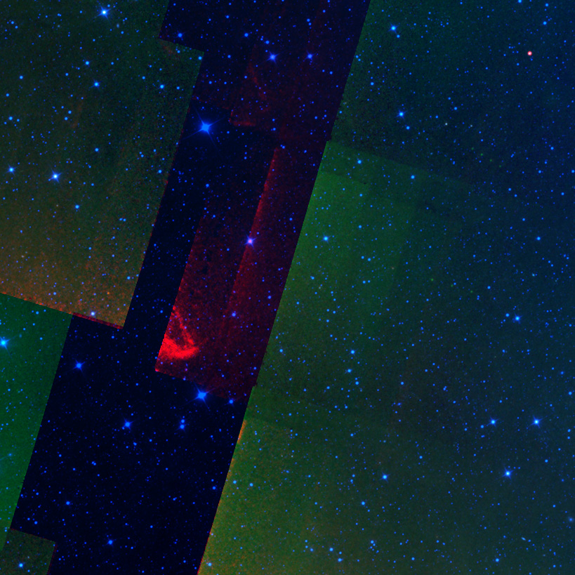
There are a few cases where most or even all of the available input frames touching parts of an Atlas Tile are within the masked region resulting in incomplete rejection of the scattered light artifacts, or, in the worst cases, zero-coverage holes in the Atlas Images and Catalog. An example of such an Atlas Image, 3165m137_ac51, is shown in Figures 20-22. Because the extent of scattered moonlight is larger in W3 and W4, the loss of coverage is more severe in those bands, and gaps where no valid data can be found are evident. In contrast to the All-Sky Data Release, the increased coverage in W1 and W2 for this AllWISE Data Release means that the coverage in W1/W2 is now enough that the outlier detection threshold is met, and so spurious features such as cosmic rays no longer contaminate these image.
| AllWISE: |
 |
 |
| W1-4 INT | W1-4 COV | |
| All-Sky: |
 |
 |
| W1-4 INT | W1-4 COV | |
| Figure 20 - Intensity and coverage images of a single Atlas tile (3165m137) at an Ecliptic latitude of around +2:45°, showing clearly suppressed depth of coverage where data are missing in both the AllWISE (top) and All-Sky (bottom) images. This Tile has a significant loss of input frames due to Moonglow. The coverage is very similar at W3 and W4 to the coverage in the earlier All-Sky Data Release wavelengths, whereas the extended duration of the data in the AllWISE release allows W1 and W2 to re-view those regions and fill in the lost coverage. | ||
 |
 |
| W1 | W2 |
 |
 |
| W3 | W4 |
| Figure 21 - Atlas Intensity Images for Tile 3165m137_ac51, showing residual scattered light and total loss of coverage in W3/W4 because of Moon contamination. The extent of influence of scattered moonlight is larger at longer wavelengths, but there is a suppression of coverage at W1/W2 caused by Moonglow in only one epoch of observing. | |
 |
 |
| W1 | W2 |
 |
 |
| W3 | W4 |
| Figure 22 - Corresponding square-root-scaled depth-of-coverage map for Atlas Image 3165m137_ac51 showing obvious Moon contamination; the depth-of-coverage ranges from ~9 near the lower left to ~22 toward the lower right in W1 and W2, and from 0 near the lower left to ~9 toward the lower right in W3/W4. | |
To assist in the proper identification of moon-contaminated Tiles, there are FITS keywords in the Atlas Image headers that describe the Moon contamination mitigation process. These are detailed below in Table 5. These parameters are also available in the Atlas Inventory metadata tables. As an example, for Tile 3165m137_ac51 in W1/W2/W3/W4, the value of MOONINP indicates that 114/149/165/165 frames (out of 304/304/191/191 initial frames per band) are flagged as "suspect" for moon-glow; of these, MOONREJ=114/149/153/143 were rejected, leaving only NUMFRMS=190/155/38/48 frames to make up the final Tiles. With such extreme ratios, care should be taken with the portions of the Tile nearest to the uncovered area. The WISE outlier detection relies on median absolute deviation as a robust measure of the dispersion of the pixel intensity distributions at any particular location. This technique becomes unreliable below a depth-of-coverage of five, so outliers may be incorrectly flagged and removed.
| Keyword | Meaning | Data Type |
|---|---|---|
| MOONREJ | Number of frames rejected due to moon-glow | int |
| MOONINP | Initial number of frames with suspect moon-glow | int |
| NUMFRMS | Final number of frames touching footprint | int |
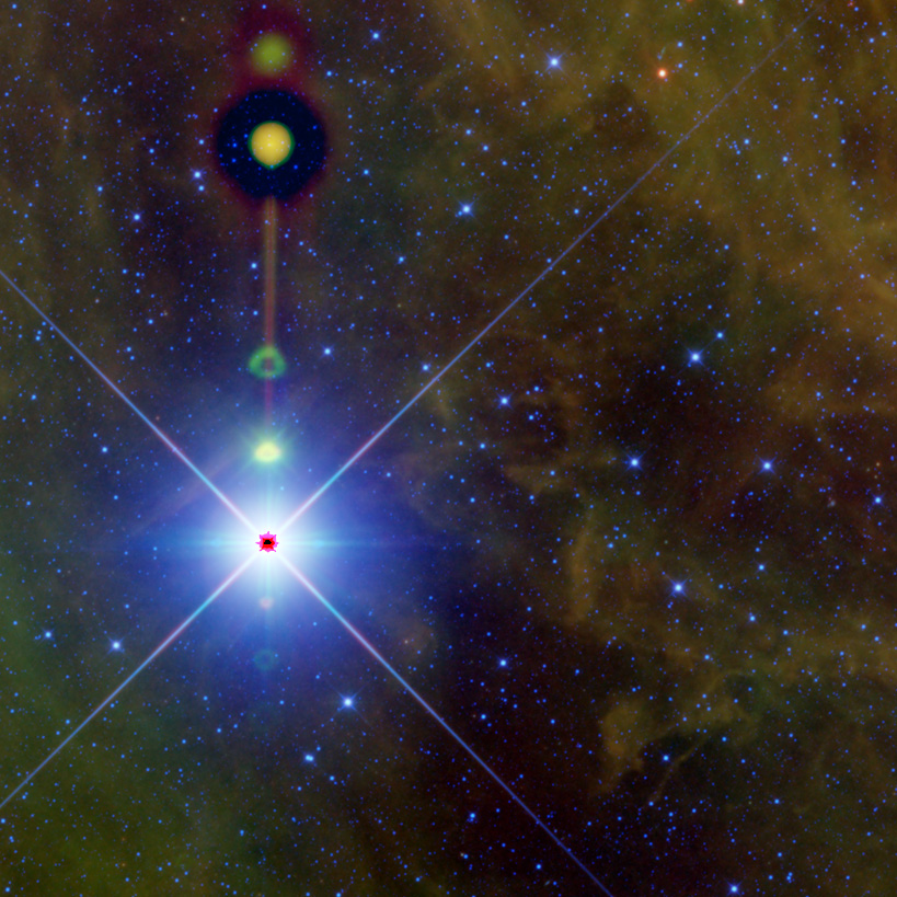
Bright stars have saturated regions of zero coverage and a suppressed depth-of-coverage in the halo. Tiles with bright stars will therefore have regions of apparent low coverage; this differs somewhat between the All-Sky Data Release and the AllWISE Data Release. This can be illustrated visually in an extreme case for a very bright star, Betelgeuse. As a roughly -4th mag star, Betelgeuse saturates thoroughly in each of the WISE bands, making it an easy example for the effect. Low coverage at the location of the star, its ghost images, and its latent image and other glints are all readily visible.
We show in Figure 23a the intensity in W1-4 for Betelgeuse from Tile 0884p075_ac51. The corresponding depth-of-coverage image in W1-4 is shown in Figure 23b.
 |
 |
| Figure 23a - Atlas Intensity Image in W1-4 for Betelgeuse from Tile 0884p075_ac51. For this very bright source, many causes of spurious or potentially spurious sources can be seen: ghosts and latents, diffraction spike objects, halo objects, etc. | Figure 23b - Atlas depth-of-coverage in W1-4 for Betelgeuse. |
Bright stars have a noticeable impact on depth-of-coverage, but also a more subtle change in sky coverage as measured by the Catalog. Very bright stars effectively obscure background sources with their their scattered light halos and diffractions spikes, and they elevate the surrounding background, thus increasing the source detection limits.
Qualitatively, this effect is the same in the WISE All-Sky Data Release. The interested reader is referred to Section VI.2.c.iii of the All-Sky Explanatory Supplement for more details.
WISE's angular resolution and sensitivity combine to provide a noticeable frequency of blended sources. While the WISE source extraction and photometry pipeline does attempt to deblend modestly extended structure into multiple sources, it cannot do this for objects at very close separations. This produces an effective limit to the window function of spatial correlations in the Catalog at very small distances.
Qualitatively, this effect is the same in the WISE All-Sky Data Release. The interested reader is referred to Section VI.2.c.iv of the All-Sky Explanatory Supplement for more details.
In regions with a large number of sources or particularly bright sources (either diffuse or point-like), the depth-of-coverage can vary between wavelengths in a spatially-varying way dependent on the intensity structure. Hence, performing tasks such as aperture photometry on extended sources must take into account these variations across the source.
Qualitatively, this effect is the same in the WISE All-Sky Data Release. The interested reader is referred to Section VI.2.c.v of the All-Sky Explanatory Supplement for more details.
Last update: 16 April 2015