SPATIAL DISTRIBUTION MODEL OF THE GALAXY
Thomas Jarrett,IPACSeptember, 1992
ABSTRACT (revised: July 14, 2000)
The number and distribution of Milky Way stars as seen in
the near to mid-infrared is modeled
using an adaptation of the Bahcall and Soneira (1980) optical
star count model. We have imployed the discrete population
formalism of Elias (1978),
Jones et al. (1981), Garwood and Jones (1987) and Jarrett (1992).
The model includes the class III (evolved giant), class IV (subdwarfs) and
class V (main sequence) stellar populations.
These are further divided into
disk and spheroid spatial distributions (ala Bahcall and Soneira).
The stars are discretely binned by their spectral types,
ranging from the hottest O stars to the coolest M dwarfs,
giving a total of 22 separate
spectral bins for the main sequence, and 12 for the luminous giants
(ranging from G2 to M7 giant). The optical/infrared colors, fluxes and
luminosity function per spectral type
are based on empirical data (e.g., Koornneef 1983; 2MASS, ISO and IRAS).
The interstellar extinction is applied as a smooth exponential
function of Galactic position, characterized by a scale height and
disk length. The model parameters were tuned using deep optical and
infrared star counts. The resultant model was validated using the
2MASS all sky infrared (1 - 2 microns) survey down to J = 15 mag and K = 14 mag
(~2 mJy).
Introduction
In this html document a description of contemporary models simulating the spatial distribution of stars in the Galaxy is presented, including a version of the "standard" model used in Jarrett (1992). Our model (and those like it) attempt to predict the stellar surface density in a given direction from the Sun. Specifically, the model predicts the total number of stars per square degree, brighter than apparent magnitude m in a direction whose Galactic coordinates are (l,b). This quantity is usually designated N(m,l,b). The stellar surface density is determined by the spatial contributions from the Galactic disk and spheroid populations. Accordingly,
In addition to disk and spheroid stars, some models include components due to a faint halo population and a "thick" disk population.
Numerical distribution models have been developed by Elias (1978) and Bahcall and Soneira (1980; henceforth B&S) assuming a purely exponential density of stars in the disk (Elias applied this model to near-infrared wavelengths) and in the spheroid (B&S added this component to their optical model). Later Jones et al. (1981) and Garwood and Jones (1987) modified the Elias (1978) model to include a spheroidal component, so that their infrared simulation resembled the B&S model.
The Stellar Distributions
Seen from the vantage point of the Sun, our home Galaxy is clearly a flattened structure, with the Solar system situated within a disk of stars, and well offset from the center of this spiral "wheel". It is more difficult to view stars above or below the Galactic disk (globular clusters are a notable exception) especially toward the Galactic center, so we must look to nearby galaxies in order to infer the distributions of other spatial components that may be important in building a model of our galaxy. De Vaucouleurs (1958; 1959; 1977) reported a spheroidal population of stars in spiral galaxies; these stars have a distribution not unlike that of elliptical galaxies that is well-approximated by a flattened exponential. This component is further divided into an inner "bulge", which can also be seen in the Milky Way at far-infrared wavelengths (cf. Habing et al. 1985), extending ~3 kpc from the Galactic center. A third component, the so-called "halo", has been proposed as a solution to the non-Keplerian, flat rotation curves observed in our Galaxy and in other spiral galaxies (cf. Bahcall 1984 for a discussion on the mass to light deficit). However, while halo stars are critical to dynamical models, their intrinsic faintness moderates their overall importance as a spatial component; thus, they are usually omitted from distribution models. We are left with a two component model of the Galaxy, containing an exponential disk and spheroid.
The Galactic Disk Contribution
The disk population is composed of a mixed ensemble of main sequence stars and evolved stars of varying mass and age. Each spectral type belonging to the dwarf and giant populations can be characterized by a scale height, which is basically an indicator of age. The older the star, the more dynamical interactions it has suffered with other stars and giant molecular clouds (Spitzer and Schwarzschild 1951). The result is an increase in the spatial velocity of older stars (particularly along the vertical axis of the disk). Along with dwarfs and giants, we include in our disk model oxygen-rich Miras, semi-regular and irregular variables, carbon stars, and AGB stars; since luminous mass-loss stars have similar photometric and spatial properties (e.g., luminosity, infrared color excess, scale- height), these stars are assembled into one population which we loosly call AGB.
At fixed Galacticentric distance, the number density of stars of spectral type s along the vertical or z direction is a function of the scale height and spectral type. For example, M dwarfs have relatively large scale heights, ~ 300 pc, in contrast to the younger A-type stars with ~ 100 pc (Faber et al. 1976). Giants and subgiants have scale-heights typically between 200 and 500 pc, though their uncertainty is greater than that of the dwarf luminosity class (cf. B&S).
Within the plane of the disk, the radial density function can be expressed in terms of the distance from the Galactic center (in the plane of the disk), the Solar distance from the center, and the Galactic disk scale length. The latter parameter varies as a function of galactic morphological type (Freeman 1970). For the Milky Way, published values of the scale length range from 2.2 to 3.5 kpc (De Vaucouleurs and Pence 1978; Knapp et al. 1978; McCuskey 1969). B&S adopt a mean value of 3.5 kpc (with R0 = 8 kpc), whereas Jones et al. (1981) treat the scale length as a free parameter ranging from 2.2 to 3 kpc (where R0 = 8.7 kpc).
The two density functions can be combined to arrive at the disk spatial density function. To transform this function into a distribution formula per spectral type, one must normalize using the appropriate luminosity functions. The luminosity function per spectral type can be modelled as a gaussian, where each spectral type has an intrinsic uncertainty in its luminosity or absolute magnitude due to calibration assumptions (i.e., discretely grouping stars together) and systematic errors within the calibration (cf. Mihalas and Binney 1981); the function includes the mean absolute magnitude per spectral type, the intrinsic dispersion and the luminosity function in the Solar vicinity (i.e., the local number density per spectral type).
The Spheroid Contribution
Following the example of de Vaucouleurs (1959), B&S characterized the spatial distribution of spheroidal stars in the Galaxy with a r1/4 exponential measured radially from the Galactic center, with re analogous to a scale length, approximately equal to R0 / 3 (de Vaucouleurs and Buta 1978). A virtue of this density formula is that it assumes spherical symmetry, while other models involve a more complex oblate symmetry (cf. King 1966). In a later paper, Bahcall and Soneira (1984) turn to an oblate distribution with an axis ratio of 0.8, to better fit the observational data.
It is by no means an easy task to determine the local luminosity function for spheroidal stars owing to the Sun's relative position with respect to the spheroid, and the rarity of these stars compared to the disk population. Stars in globular clusters are often used to compare with (or add to) those of the field spheroid ensemble. Schmidt (1975) was able to isolate a sample of sub-dwarf stars, presumably belonging to the spheroid population, because of their remarkable space velocities (100 to 250 km s-1). Although the statistics are poor, Schmidt computed the resultant luminosity function and found that the general shape of the luminosity function belonging to the high proper motion stars resembles that of the disk. The overall number density is, however, about 3 orders of magnitude smaller. Combining the data of Schmidt (1975) and Wielen (1974) with the star count data of Bahcall and Soneira (1980), the spheroidal luminosity function is best described using the shape of the disk luminosity function, normalized with a value between 500-1 to 800-1 (Bahcall, Schmidt and Soneira 1983), where the larger value corresponds to a spheroid with oblate symmetry.
A Thick Disk?
It should be noted there is a fair amount of controversy as to the overall nature of the spheroid population. Gilmore and Reid (1983) claim that many high proper motion stars are in fact a tracer of a thick disk component. They point out that if one increases the disk scale heights ( ~ 1500 pc), the resultant distribution matches that of the subdwarf stars. Their stellar surface density simulations include the disk and spheroid populations, as well as a third, "intermediate" population which contains metal-poor subdwarf stars with a z-distribution characteristic of a thick disk (Reid 1983). However, Bahcall and Soneira (1983; 1984) maintain that Gilmore and Reid did not include evolved spheroid stars in their simulation, consequently arriving at a false conclusion. These giant stars are very bright and very far away from the Sun. If one mistakenly identifies them as dwarfs, their intrinsic brightness is vastly changed, the result being that their placement is ~1000 pc off the disk mimicking a thick disk as opposed to ~10 kpc where the giants would lie.
Gilmore and Reid question the overall abundance of evolved spheroid giants, suggesting that selection effects may be deceiving their true numbers. Nonetheless, Bahcall and Soneira (1984) are confident the observational evidence for these subgiants is firm (cf. Ratnatunga 1982). The fact remains that the B&S model adequately simulates the observed Galactic distribution in several diverse directions (see Section 4), proving the robust nature of the two-component model. The existence of a thick disk shall probably remain in the sphere of debate for some time. The reader is referred to a spirited discussion between the two camps in a talk by Bahcall and Soneira (1983), and to the comprehensive review by Gilmore, Wyse, and Kuijken (1989) in which the authors argue based on the most recent observational evidence for the existence of a thick disk.
Interstellar Extinction
A final ingredient to consider in modelling surface density is interstellar extinction. Starlight is absorbed by grains of dust and light at shorter wavelengths is preferentially blocked, resulting in a selective reddening of the starlight. The spatial distribution of dust is usually modeled similarly to that of the young disk population, namely, an exponential with a scale height severely restricted to the plane of the disk (~100 pc; Spitzer 1978). Jones et al. (1981) expanded this relation to include an absorption scale length in the disk, which they determine to be ~ 4 kpc. and a normalization constant corresponding to the local absorption in magnitudes per kpc. The canonical value is typically quoted between 1 and 2 mag kpc-1 at visual wavelengths (cf. Elias 1978). The absorption function described above does not take into account dense clumps arising from molecular clouds and giant molecular clouds in the disk. This omission may become a problem when modelling the stellar distribution at low galactic latitudes (b < 10).
Model Developed in this Work
In the following discussion, a version of the model described above used in the dissertation of Jarrett (1992) is outlined. Numerical simulations are carried out to validate the model with the results of B&S and real data. The results are described in the section that follows.
Begin by transforming the number density equations into a frame centered about the Sun. Recall that it is measured from the Galactic center in the plane of the disk, and that R is measured from the Sun to the source (or viewing direction).
B&S define the luminosity, scale height and local density parameters for each spectral type in analytic form as a matter of numerical convenience. In this study, a discrete format using the values in Elias (1978), Jones et al. (1981) and Garwood and Jones (1987) is applied. This allows for more flexibility in modifying or adding new spectral types to the sample. For example, the Wielen luminosity function is added to account for the late M-dwarfs (Mv > 13 mag); also included is a Hawkins and Bessell (1988) upturn in the luminosity function at the very faint end (Mv > 16), which can be compared with the nominal values given by Wielen. The models developed by Elias, Jones et al., and Garwood and Jones are specifically applied to K-band (2.2 micron) data. The transformation involves color corrections (i.e., V - K) and interpolation of the luminosity function. In the case of evolved stars, the V-band luminosity function given in Mamon and Soneira (1982) is used. The scale height and absolute magnitude dispersion values given by Garwood and Jones remain the same. Table 1 lists the spectral type, brightness, colors, local number density, dispersion and scale height. The optical colors are in the Kron-Cousin system (from Bessell 1990), and the infrared colors are from Koornneef (1983). The spheroid population has the same parameters except their number density decreases by a factor of 800, and owing to their intrinsic metal poor composition, their colors tend to be blue with respect to main sequence dwarfs.
The spatial distribution model embodies a numerical algorithm that follows 4 basic steps: 1) integrate the surface density functions for each spectral type over a differential volume defined by stepping an incremental distance through the viewing cone (that is, a volume bounded by a specified field of view, whose direction is given by the Galactic coordinates), 2) assign the appropriate mean absolute magnitude and its dispersion to the stars given by step 1, 3) compute the total interstellar absorption within the volume by integrating the extinction surface density function, and 4) calculate the apparent brightness, 5logd - 5 + A + M, for each star given by step 1. It is then a simple matter to derive colors and construct cumulative star counts curves.
Consider the disk population. Integrate the density function out to some distance d, with NT being the total number of stars of spectral type s contained in the cone volume extending distance d. We do not need to waste computer time integrating the luminosity function over a wide range in magnitude. Instead, we solve for absolute magnitude based on the gaussian luminosity distribution, characterized by the mean absolute magnitude and the intrinsic magnitude dispersion, via a Monte Carlo technique. Next integrate the density function out to a distance d + delta(d) and integrate the interstellar absorption function. The apparent magnitude is given by the distance modulus. For example, where d* is measured in kpc, AR and AI are derived using reddening curves and the ratio of total to selective extinction. The apparent (reddened) colors are calculated using the above magnitudes. In addition, we may apply a random error to the colors, which will mimic uncertainties due to signal to noise, poor seeing conditions and calibration to standard colors.
The simulation using a spheroid component follows the same procedure. Integrating the density function. Compute the number difference, apply an extinction and color correction. It should be noted that the volumes are integrated out to some maximum distance depending on the direction the model is attempting to simulate. Bahcall, Schmidt and Soneira (1983) tabulate Rmax as a function of galactic coordinates (see Table 1 in their paper). This value is constrained by the requirement to clearly separate the two major stellar components, the disk and spheroid. For the disk, the maximum distance to which the surface density function is integrated depends on the Galactic coordinates and geometry of the disk. Here we are assuming a perfectly flat, circular disk of thickness 2zH, and diameter 2X. The Milky Way Galaxy appears to have a total diameter of about 25 kpc (cf. Bok 1979) and, based on stellar spatial scale heights, a thickness of about 2 kpc or so. The maximum distance, dmax, is given within the geometric relation, unless zmax is greater than zH.
Validating the Model
In this section, a brief description of numerical tests conducted by Bahcall and Soneira (1984) in five different fields is presented. Simulations are performed using the model described in the last section for the fields: 1) north Galactic pole (NGP); 2) SA 57: l = 65, b = 86; 3) SA 68: b = -46, l = 111; 4) Aquarius: b = -57, l = 36; and 5) SA 51: b = +21, Galactic anticenter, comparing these results with those of Bahcall and Soneira, and real data. The fields were chosen by Bahcall and Soneira to minimize confusion and interstellar extinction (i.e., by avoiding locations anywhere near the plane of the Galaxy), as well as to test the degree of oblateness in the spheroid. Finally, additional fields are considered and the results are compared with infrared data from the 2MASS Protocam. The fields lie in the directions of the Galactic plane (l = 53 and 140, b = 0), toward M92 (l = 68, b = 34), and the NGP.
Both SA 57 and the NGP offer an excellent test of the spheroid parameters because disk stars are considerably less numerous well off the plane, whereas spheroid stars can be seen several kpc from the Sun. Bahcall and Soneira were able to fit their simulated differential starcounts to the data with better than 20% accuracy. They found that spheroid stars begin to dominate the total number observed at visual magnitudes fainter than ~17. Disk giants diminish rapidly beyond V ~ 12, and disk dwarfs vanish at V ~ 25. In Figures 1a and 1b plots of the differential starcounts using the model described in Section 3 is shown for these two regions. The total contribution is drawn with a solid line, disk dwarfs are shown with a short dashed line, disk giants with a dotted line, and the total contribution due to the spheroid population is drawn with long dashed line. Real data is represented by filled circles. In Figure 1a it is apparent that the predicted starcounts fit the data by Reid and Gilmore (1983) with an accuracy ~10% for visual magnitudes fainter than 10. At the bright end the fit begins to deviate substantially, due in part to Poisson statistics. This effect can be seen in Figure 1b as well, where the predicted counts do not follow a smooth line or the data of Weistrop (1972). Overall the fit in Figure 1b is good to ~20%, where some deviation settles in at V > 16 mag. As in the case with the B&S model fits, it can be seen that the spheroid stars begin to dominate the total numbers beginning at V ~ 17. The dominant spectral component in the spheroid population are distant K giants.
As we move down in galactic latitude, the importance of spheroid stars lessens relative to disk dwarfs. This effect can be seen in Figures 2a (SA 68) and 2b (Aquarius). The main difference between the two plots is that the direction of Aquarius lies substantially closer than SA 68 to the Galactic center; consequently, more spheroid stars are seen (cf. the "bulge" sub-component of the spheroid). In the case of SA 68, the model fits the data (taken from Bahcall and Soneira 1984) to an accuracy of 10 - 25%, which is about the accuracy of the photometry itself. The predicted counts for Aquarius have an even better fit, ~10%, with only two data points deviating by about 20% (Tritton and Morton, 1983, taken from Bahcall and Soneira 1984). Likewise, B&S were also able to fit the predicted starcounts to the data with accuracies better than 20%.
Finally, consider the case of SA 51. In Figure 3, a plot of the predicted differential starcounts versus observed data (by King, taken from Bahcall and Soneira 1984) is shown. Notice that at low galactic latitudes the total number density increases, while the contributions due to disk giants and spheroid stars substantially decreases. The fit is accurate to ~20% between 12 < V < 21, with greater deviation occurring at the bright end, (again, due to statistics) and the faint end, where only ~30% accuracy is achieved. The model fits by B&S do a little better at the faint end, with 20% accuracy.
To summarize: both the B&S and the optical spatial distribution model of this study adequately fit, to the accuracy of the observational data, starcounts in five different Galactic fields. The fact that these fields are located toward diverse galactic latitudes and longitudes attests to the robustness of the models. The models can thus be applied, with a satisfactory degree of confidence, toward most fields above the galactic plane. Beyond these limits there is uncertainty, since no tests were performed by Bahcall and Soneira.
Simulations using the infrared parameters provide similar (re: encouraging) results as those presented above. The NGP model simulations agree quite well with the Protocam data (which has photometric accuracy of 10 - 20%), as seen in Figure 4. Within the Galactic plane the model results (Figures 5 and 6) appear to match the true stellar distributions as evident from the Protocam data (in the luminosity range in which the data is complete). The success of the model in this spatial regime is perhaps surprising given the extreme source density (two orders of magnitude greater than that of the NGP) and the rather simplistic assumptions of the model. Be that as it may, the model results clearly show that evolved stars, and in particular AGB stars (see Figure 5), dominate the total star counts contributed by the aggregate disk population. It is interesting to note that the field in the direction of l = 140 is cloaked by a molecular cloud that lies some 2.2 kpc from the Earth. The cloud acts as a semi-opaque screen, with visual extinctions ranging from a few to perhaps 50 mag. We have included in our model an opaque `wall' located 2.2 kpc from the Sun possessing an average extinction of AV = 10 . From Figure 6 it can be seen that the cloud tends to dampen the source counts of distant, luminous evolved stars, while having little effect on the dwarfs (since they are mostly foreground to the cloud). The total yield in source counts agrees to within 10% of the data observed using the SQIID array.
For higher Galactic latitudes (b > 10), the faint source counts are dominated by F - K dwarfs. Consider the high Galactic latitude field toward the M92 globular cluster (b ~ 34). Figure 7a shows the model results along with the Protocam data which includes sources from the globular cluster. Figure 7b is the same as 7a except that the M92-associated stars have been subtracted from the Protocam data. Again, the simulations adequately match (to within 10-15%) the field star population toward the Hercules constellation (Figure 7b).
It should be noted that the photometric data provide information regarding the total cumulative star counts, but do not discriminate between various spectral types and luminosity classes. In most cases it is not possible to test the validity of the relative fraction of dwarf to giant to spheroid stars that is provided by the spatial distribution models.
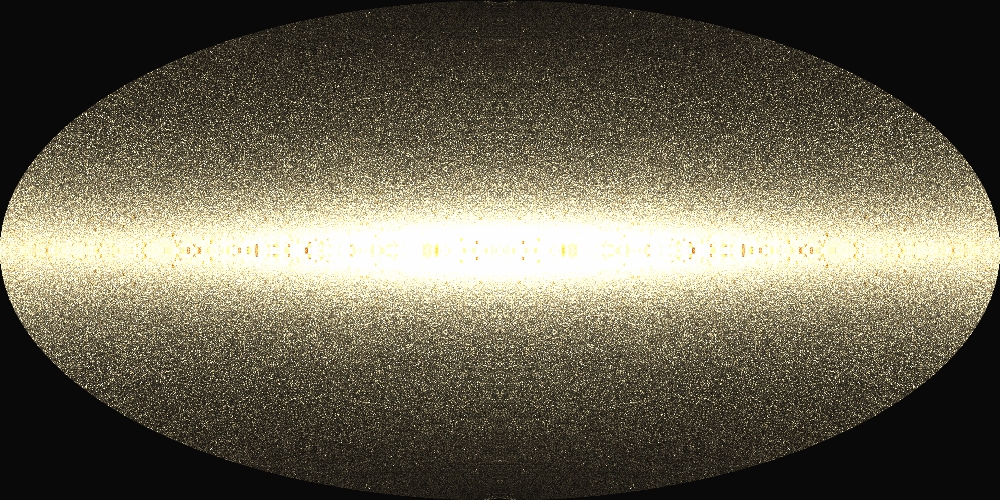
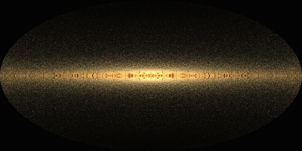
The Infrared All-Sky
Bahcall, J.N. 1984, Ap. J., 276, 169.
Bahcall, J.N., Schmidt, M., and Soneira, R.M. 1983, Ap. J., 265, 730.
Bahcall, J.N. and Soneira, R.M. 1980, Ap. J. Suppl., 44, 73.
Bahcall, J.N. and Soneira, R.M. 1983, in The Nearby Stars and the Stellar Luminosity Function, ed.
A.G. Davis Philip and A.R. Upgren (Schenectady: L. Davis Press), p. 209.
Bahcall, J.N. and Soneira, R.M. 1984, Ap. J. Suppl., 55, 67.
Bessell, M.S. 1983, Publ. Astron. Soc. Pac., 95, 480.
Bessell, M.S. 1986, Publ. Astron. Soc. Pac., 98, 1303.
Bessell, M.S. 1990, Astron. Astrophys. Suppl., 83, 357.
Bessell, M.S. 1991, A. J., 101, 662.
Bless, R.C. and Savage, B.D. 1972, Ap. J., 171, 293.
Bok, B.J. 1937, The Distribution of Stars in Space (Chicago: University of Chicago Press).
Bok, B.J. 1956, A. J., 61, 309.
Code, A.D. and Bless, R.C. 1970, in IAU Symp. 36, p. 173.
Dahn, C.C., Liebert, J., and Harrington, R.S. 1986, A. J., 91, 621.
DeVaucouleurs, G. 1958, Ap. J., 128, 465.
DeVaucouleurs, G. 1959, in Handbuch der Physik, 53, ed. S. Fluegge (Berlin: Springer-Verlag),
p. 311.
DeVaucouleurs, G. 1977, Astron. Astrophys., 56, 91.
DeVaucouleurs, G. and Buta, R.J. 1978, A. J., 83, 1383.
DeVaucouleurs, G. and Pence, W.D. 1978, A. J., 83, 1163.
Dickman, R.L. 1978, A. J., 83, 363.
Elias, J.H. 1978, Ap. J., 223, 859.
Elias, J.H. 1978, Ap. J., 224, 453.
Elias, J.H. 1978, Ap. J., 224, 857.
Faber, S.M., Burstein, D., Tinsley, B.M., and King, I.R. 1976, A. J., 81, 45.
Freeman, K.C. 1970, Ap. J., 160, 811.
Garwood, R. and Jones, T.J. 1987, Publ. Astron. Soc. Pac., 99, 453.
Gilmore, G. and Reid, N. 1983, Mon. Not. Roy. Astron. Soc., 202, 1025.
Gilmore, G., Wyse, R., and Kuijken, K. 1989, Ann. Rev. Astron. Astrophys., 27, 555.
Greenberg, J.M. 1968, in Nebulae and Interstellar Matter, ed. L.H. Aller and B.M. Middlehurst
(Chicago: University of Chicago Press), p. 221.
Habing, H.J., Olnon, F.M., Chester, T.J., Gillett, F.C., Rowen-Robinson, M., and Neugebauer, G.
1985, Astron. Astrophys., 152, L1.
Hawkins, M.R.S. and Bessell, M.S. 1988, Mon. Not. Roy. Astron. Soc., 234, 177.
Herbst, W. and Dickman, R.L. 1983, in The Nearby Stars and the Stellar Luminosity Function, ed.
A.G. Davis Philip and A.R. Upgren (Schenectady: L. Davis Press), p. 187.
Jarrett, T.H., 1992, Ph.D. Thesis, University of Massachusetts.
Johnson, H.L., Mitchell, R.I., Iriarte, B., and Wisniewski, W.Z. 1966, Comm. Lunar and Planetary
Lab., 4, 99.
Jones, T.J., Ashley, M., Hyland, A.R., and Ruelas-Mayorga, A. 1981, Mon. Not. Roy. Astron. Soc.,
197, 413.
Jones, B.F. and Herbig, G.H. 1979, A. J., 84, 1872.
Jura, M. and Kleinmann, S.G. 1992, Ap. J. Suppl., 83, 001.
Jura, M. and Kleinmann, S.G. 1989, Ap. J., 341, 359.
King, I.R. 1966, A. J., 71, 131.
Knapp, G.R., Tremaine, S.D., and Gunn, J.E. 1978, A. J., 83, 1585.
Koornneef, J. 1983, Astron. Astrophys., 128, 84.
Leggett, S.K. and Hawkins, M.R.S. 1988, Mon. Not. Roy. Astron. Soc., 234, 1065.
Mamon, G.A. and Soneira, R.M. 1982, Ap. J., 255, 181.
McCuskey, S.W. 1969, A. J., 74, 807.
Mihalas, D. and Binney, J. 1981, Galactic Astronomy (San Francisco: W.H. Freeman and Company).
Miller, G.E. and Scalo, J.M. 1979, Ap. J. Suppl., 41, 513.
Ratnatunga, K.U. 1982, Proc. Astr. Soc. Australia, 4, 422.
Reid, N. 1987, Mon. Not. Roy. Astron. Soc., 225, 873.
Reid, N. 1991, A. J., 102, 1428.
Reid, N. and Gilmore, G. 1982, Mon. Not. Roy. Astron. Soc., 201, 73.
Savage, B.D. and Mathis, J.S. 1979, Ann. Rev. Astron. Astrophys., 17, 73.
Scalo, J.M. 1986, Fund. Cosmic Phys., 11, 1.
Schild, R.E. 1977, A. J., 82, 337.
Schmidt, M. 1975, Ap. J., 202, 22.
Spitzer, L. 1978, Physical Processes in the Interstellar Medium (New York: Wiley).
Spitzer, L. and Schwarzschild, M. 1951, Ap. J., 114, 385.
van de Hulst, H.C. 1949, Rech. Astron. Obs. Utrecht, 11, part 2.
Weistrop, D. 1972, A. J., 77, 366.
Wielen, R. 1974, in Highlights of Astronomy, 3, ed. G. Contopoulos (Dordrecht: D. Reidel), p. 395.
Wielen, R., Jahreis, H., and Krueger, R. 1983, in The Nearby Stars and the Stellar Luminosity
Function, ed. A.G. Davis Philip and A.R. Upgren (Schenectady: L. Davis Press), p. 163.