
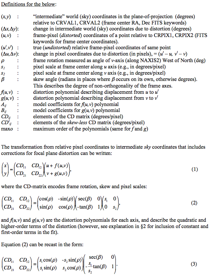
| Distortion Calibration and Code-V Modelling | |
Below we outline a method for calibrating distortion, its representation in FITS headers, and present some results from a Code-V distortion model for band 1 provided by Roy Esplin on April 28, 2008.
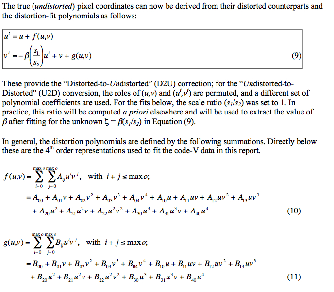
(1.) Attempting to solve for the model parameters via chi-square minimization (our method) results in a nonlinear system of equations if skew is included directly as just another parameter whose value we seek to obtain. Holding skew constant allows the system to be linear, simplifying the solution; this is not necessary for the B10 coefficient in Equation (11), indicating a lack of equivalence between these two parameters.
(2.) Because of (1) the algorithm operates by setting the skew to zero, solving the linear system for the 30 coefficients, and then having those values allows the skew to be computed; this value of the skew is then used instead of the initial guess of zero, and the linear system is solved again (actually, the skew is averaged with the previous iteration's value; damped convergence has been found desirable, since oscillations by a constant amount are observed otherwise). In this way, the full set of parameters (31 of them) are computed iteratively.
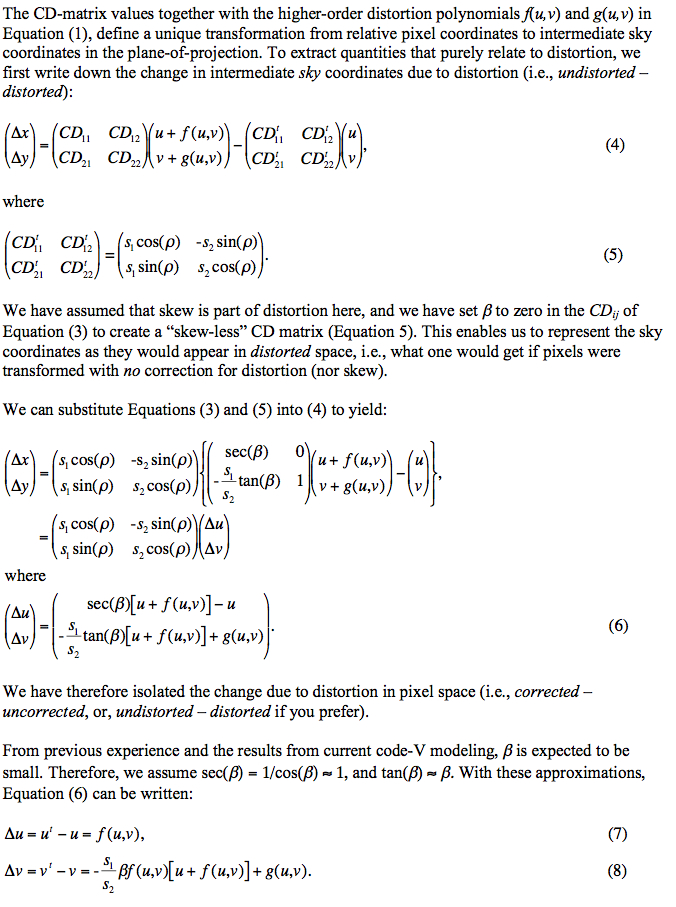
(3.) The iteration ceases when the skew is converged, where the convergence criterion is that either (a.) the relative change in skew is less than 1.0e-9; or (b.) the average of the absolute values on two consecutive iterations is less than 1.0e-15 after at least 10 iterations (the latter is needed because the skew may get so close to zero that a relative change is numerically unstable). If skew were redundant, one would expect the first solution with zero skew to be already converged, but at the mirror extremes, we find that a significant non-zero skew emerges and does converge, behavior which one expects of a meaningful parameter. This iterative approach, beginning with zero skew, clearly depends on the skew being rather small, which fortunately it is.
(4.) While the B10 coefficient multiplies u, a parameter on the ut-type axis, u is not linearly coupled to ut, which is what beta (the skew) multiplies, and so it cannot perform quite the same job. Equation (9) appears to be a linear relationship between ut and u, but the f(u,v) term is a nonlinear function of u, making ut one also. The fact that u and ut are nonlinear functions of each other removes any equivalence between B10 and the skew. There is also a coupling between the A and B coefficients that is not visible in the equations wherein they are used; in fact one might wonder why a 30x30 system is involved, since it appears that two 15x15 systems would suffice once the skew is handled separately; the reason is that the chi-square that is being minimized includes the covariances of the position uncertainties, coupling the two axes. So B10 is affected by what goes on on both axes (in principle; in fact it's probably negligible).
(5.) The skew does make for asymmetry in the way u and v are handled, but some asymmetry is unavoidable when the axes are in fact skewed, and an arbitrary choice of which axis gets to absorb the lack of orthogonality must be made.
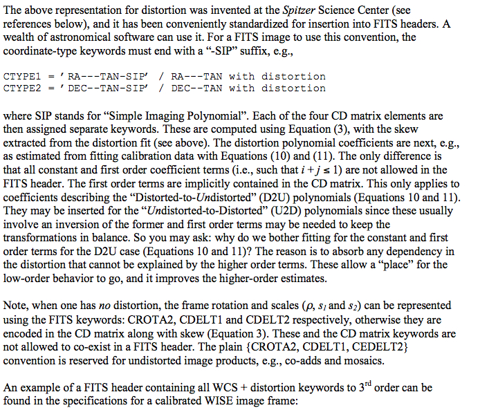
Code-V ray-trace models were provided for band 1 at the center of the scan (scan mirror angle equal to 0°), at the plus scan limit (scan mirror angle equal to +1.302°), and at the negative scan limit (scan mirror angle equal to -1.302°). The code-V data was fit with a 4th order polynomial (Equations 10 and 11).
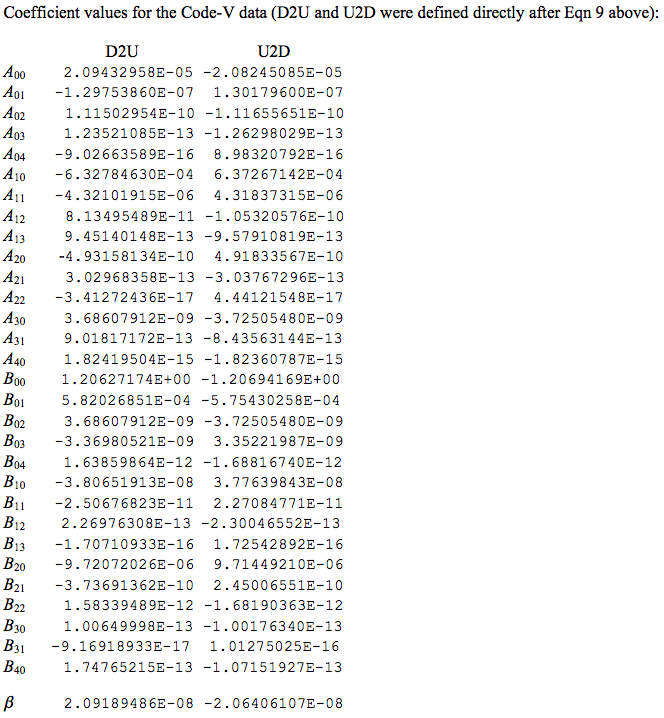
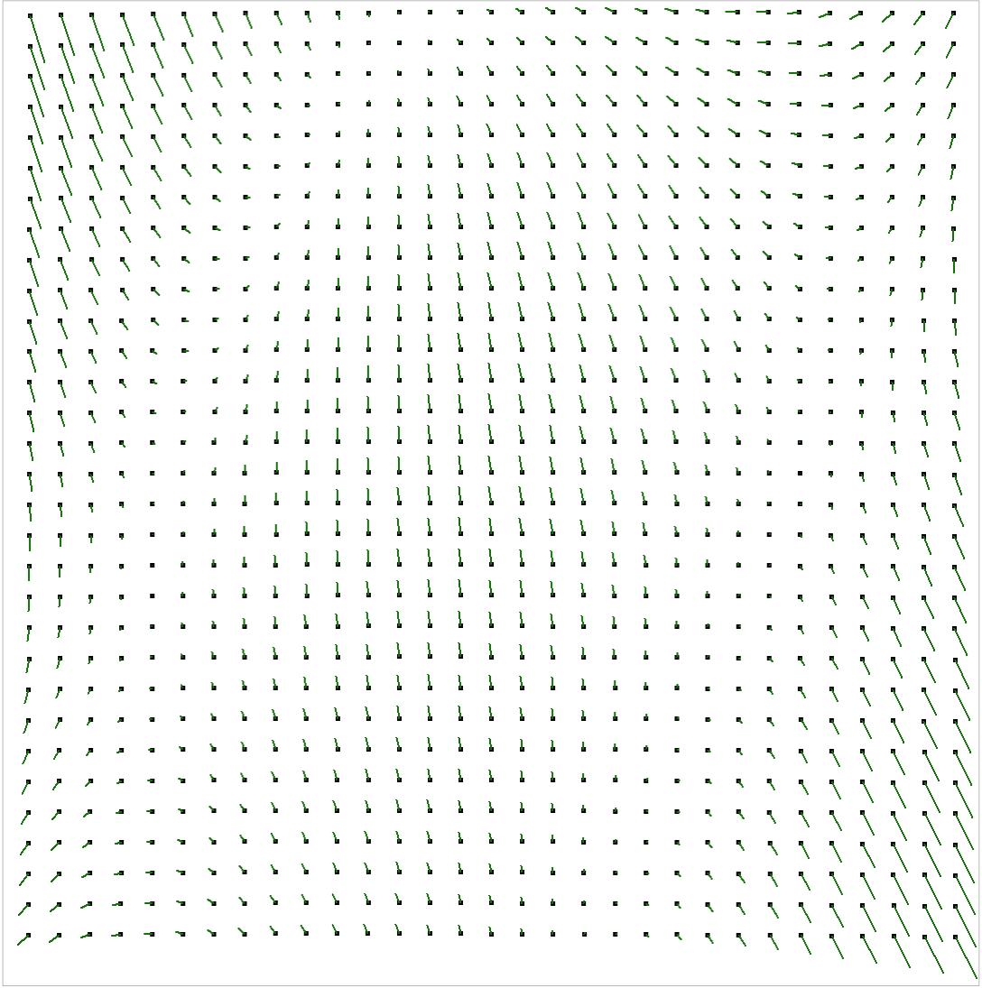
Each set of three positions of a given distorted point [with matching undistorted truth] in the x,y frame corresponding to the three mirrors positions are averaged before being fit. This resembles the scan-averaged case that will apply in the nominal survey, where a frame exposure will effectively contain information from all mirror positions. The undistorted (true) reference positions will be provided by an astrometric catalog, e.g., 2MASS. The fit coefficients are shown below, and the distortion vector map is shown in Figure (1a). The black lines show the actual averaged distortion and are three pixels wide so that they won't be obscured by the red lines, which are one pixel wide and show the model output.
This is an attempt to check whether the model will track the distortion of source centroids that are computed from exposures over the full standard travel of the scan mirror. Such centroids will probably not fall on this average position, but the small differences between these averages and the actual centroids should be negligible with respect to the model's capability. The actual centroid positions will probably be dominated by source extraction error, which should be of the same order of magnitude as the approximation herein using the averaged positions as single centroid positions.
The main conclusion is that the model should have no trouble tracking centroid displacements due to distortion if reality and Code-V are in the same ballpark.
 |
| Figure 1a - Distortion vectors averaged over all three mirror positions. For each array sample location, the three WISE-array (distorted) positions were averaged; these average positions, together with the corresponding "true" positions were then processed to compute a standard 4th-order polynomial model. The "true" positions are shown as black dots (5 x 5 array pixels in size). Thick black lines are the actual distortion of the averaged WISE-array position. Thin red lines are the model output distortion. The magnitude of distortion displacement is magnified by a factor of 15. Click on panel to enlarge. |
Figures (1b) - (1d) show distortion maps with the scan-mirror at each of the
three positions.
 |
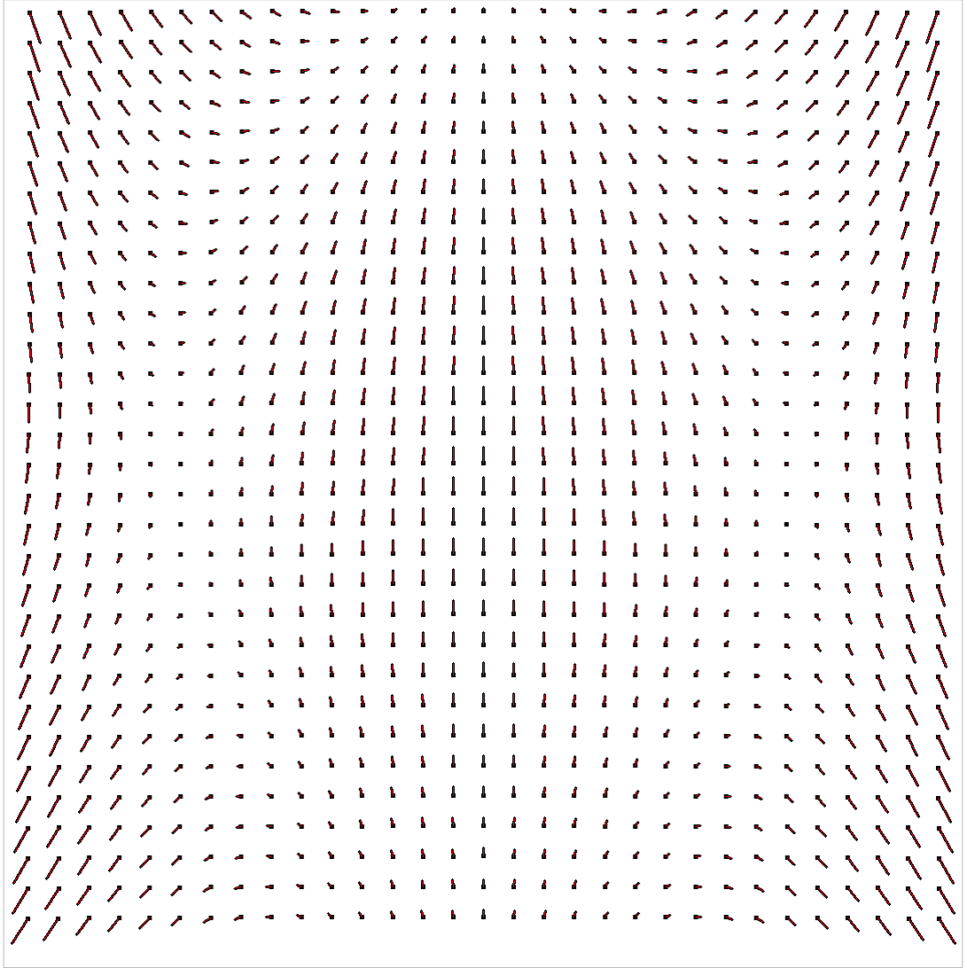
| Figure 1b - Distortion with scan mirror at center position. Black dots are array sample positions, black lines are Code V distortion, red lines are 4th-order polynomial fit values. The black lines are two pixels wide so that the one-pixel-wide red lines don't eclipse them completely. The fact that both are visible is due to that, not fitting error. Click on panel to enlarge. |
 |
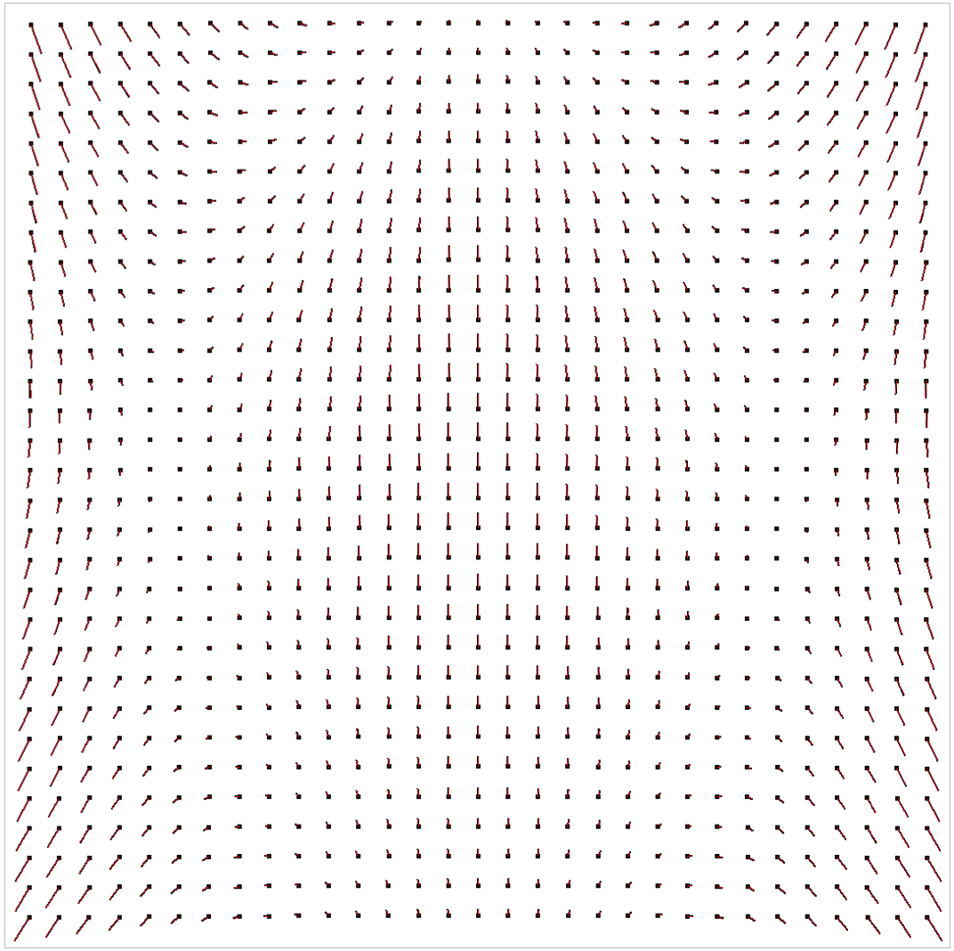
| Figure 1c - Distortion with scan mirror at the -1.302° position. Black dots are array sample positions, blue lines are Code V distortion. Click on panel to enlarge. |
 |
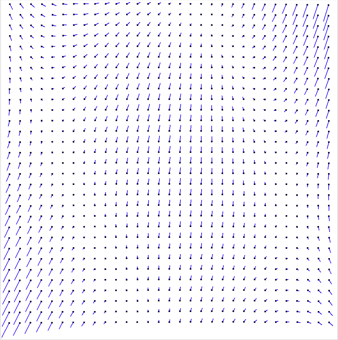
| Figure 1d - Distortion with scan mirror at the +1.302° position. Black dots are array sample positions, green lines are Code V distortion. Click on panel to enlarge. |
To illustrate the impact of skew (β) in the fits,
Figure (1e) shows the
Y-coordinate distortion fit residuals (pixel units) for
the positive-limit mirror position.
The blue dots are the standard 4th-order polynomial. The red dots are the
polynomial without any skew parameter taken into account, i.e., employing
the single-pass (no iteration necessary) polynomial coefficients with skew
set to zero.
The standard fit has residuals that are mostly zero to milli-pixel precision, some are ±0.001, and 14 points have ±0.002 residuals. Without skew, the residuals approach ±0.1 pixel. The Y residuals are shown; X is much less sensitive to skew, and the X residuals are not substantially different between the two cases, resembling the blue Y residuals.
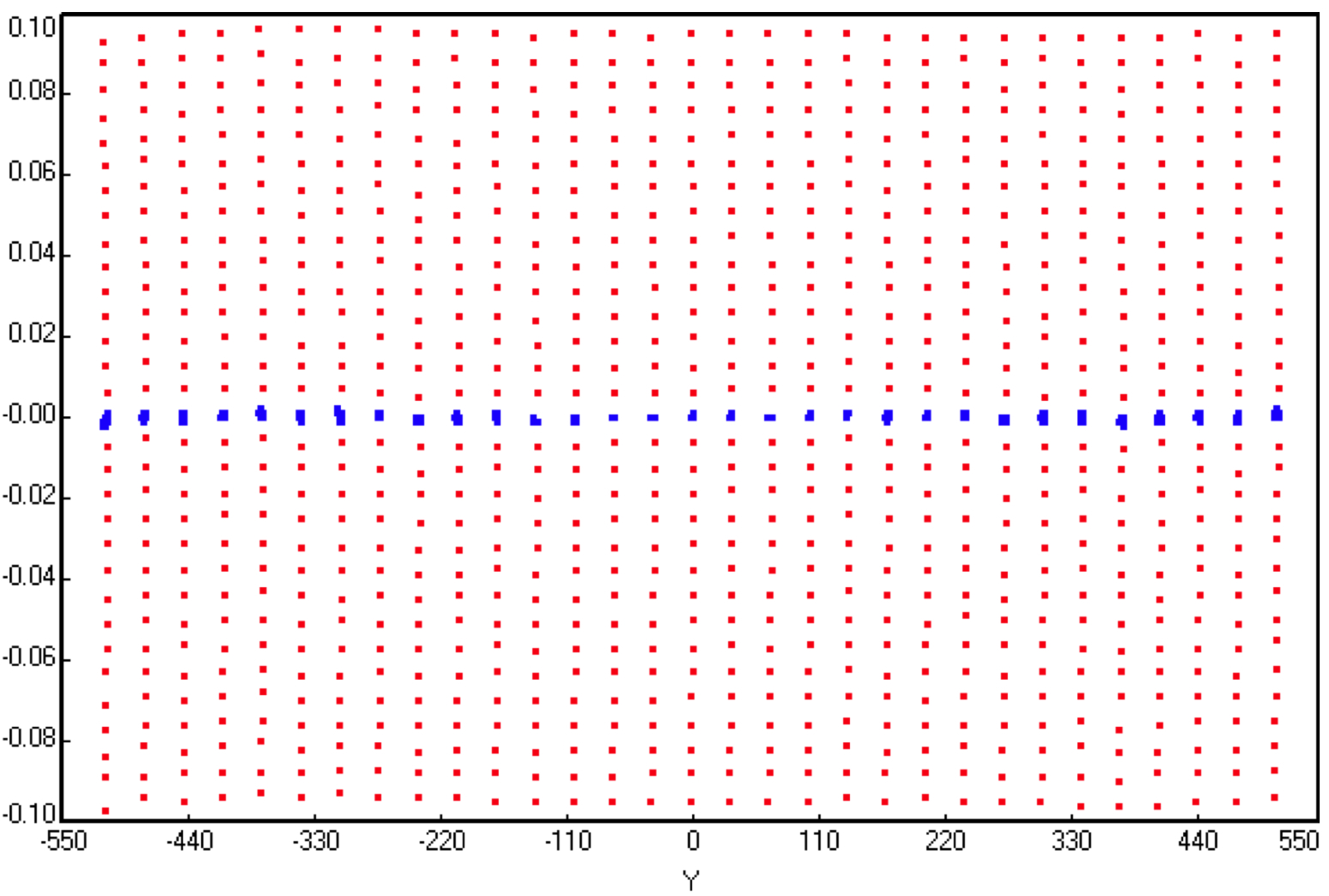 |
| Figure 1e - Distortion Fit Residuals for the +1.302° mirror position. Blue residuals are the standard 4th-order polynomial including skew; Red residuals are the 4th-order polynomial fit excluding a skew dependence. Click on panel to enlarge. |
 |
| Figure 2 - Distortion as parameterized by the 4th-order polynomial fits. The z-axis represents the magnitude of the distortion vector: Dst = [(Dx)2 + (Dy)2]1/2, where Dx = f(u,v) and Dy = g(u,v) are the components that were separately fit. x,y (as in all the plots below) are pixel coordinates relative to the frame center, and are the same as u,v in the notation above. Fits were performed to an average of the Code-V data over all mirror positions. |
 |
| Figure 3 - Same as Figure 2 but viewed in the y-z plane. |
 |
| Figure 4 - Same as Figure 2 but viewed in the x-z plane. |
 |
| Figure 5 - Fit residuals in the Dx components over array: f(u,v) − Code V displacement (ut - u). Residuals in the Dy components are similar. |