


Contents
V.3.b.ii.Adding Small Linear Motion Terms to the Source Measurement ModelSource position estimation was augmented by adding linear-in-time motion to the observational model. The previous model continues to be used in what is now called the "stationary fit." The augmented model is called the "PM fit," where "PM" originally referred to proper motion, but in fact many moving sources are close enough for parallax to contribute significantly to timedependent apparent sky position, especially because of the WISE observational mode of scanning very close to 90 degrees off of the sun vector (see section II.6.d.i). The tag "PM" has become ingrained, so the phrase "proper motion" continues to be used but should be considered only a loose-sense tag, not a literal reference to true proper motion.
The use of both fits is called the "dual solution." The stationary fit is performed first, and the full set of photometric parameters is computed. The PM fit begins with the stationary position as the initial position estimate at a fiducial time which is computed for each source as a flux-weighted mean observational epoch. Because of the effects of noise on the nonlinear chi-square minimization algorithm, it is sensitive to the initial estimates used to start the search for the minimum, and of several ways to weight the epoch averaging, flux weighting based on the stationary-fit single-frame flux solutions was found to be the most effective in reproducing motions of known moving objects. The set of photometric parameters computed for the PM fit is a small subset of that for the stationary fit (see section II.1.a.)
V.3.b.ii.1. Review of the Stationary Model
The All-Sky observational model is
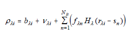 | Eq. 1 |
where ρλi is the flux in the ith usable observed pixel at the position given by the 2-vector rλi in the wavelength band λ,sn is a 2-vector giving the position of the nth blend component, fλn is the flux of the nth component, Hλ(r) is the PSF, bλi is the local background estimated in an annulus around the detected source position, and vλi is the noise in the ith pixel, with prior noise variance σ2iλ, which includes uncertainty due to the PSF model based on an initial flux estimate from aperture photometry.
The reduced chi-square figure of merit is defined as
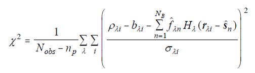 | Eq. 2 |
where Nobs is the total number of usable pixels, and the circumflexes on fλn and sn indicate that current estimates of these values are used to evaluate chi-square. These are the parameters to be estimated via minimization of chi-square, and hence the solution depends on finding the minimum in the np-dimensional parameter space. The solution proceeds as in all non-linear fitting problems: zeroth-order estimates are used to evaluate the function and its derivatives with respect to the fitting parameters, and then an extremum-finding algorithm is applied. Since chi-square is to be minimized, we seek a minimum, and the algorithm of choice is the gradient descent method (see section V.3.b.ii.3 below).
Once the minimum chi-square has been found, the primary component is output and the other solutions are discarded. The only exception to this involves active deblending. The source ensemble starts out composed of a primary component and nearby sources that were detected on the co-adds. The solution for the ensemble is called passive deblending. If the chi-square for that solution is too high, an attempt is made (subject to controllable thresholds) to find another source in the neighborhood that was not detected on the co-adds but is blended with the other ensemble sources. The details of this processing are discussed in section IV.4.c.iii of the All-Sky Release Explanatory Supplement. The bottom line is that if the reduced chi-square for the ensemble can be made smaller (by another controllable threshold) by including the new source, then it is kept and called an actively deblended source. Since this source is not in the list of coadd detections, it will not come up later as a primary component, and so it is output immediately after the primary component. Although it is theoretically possible to have more than one actively deblended component, in practice only one per blend group was permitted, and the number of secondary passive-deblend components was limited to two.
V.3.b.ii.2 Addition of Motion Estimation
The change made to the stationary observational model to produce the PM model in the AllWISE version of WPHOT is to replace sn for the primary component with a frame-dependent position that is a linear function of time. Since the primary component is usually component number 1 in the ensemble, for notational convenience we will just assign it n = 1 herein. Then
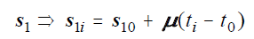 | Eq. 3 |
where s10 is the position of the primary component at a fiducial time t0, μ is the 2-vector whose elements are the linear time coefficients of the apparent motion of the primary component, and ti is the time tag for the frame in the co-add stack that contains pixel i.
The initial estimates for the components of μ are zero. These will evolve to non-zero values if this reduces chi-square. The influence of the motion on chi-square is through its displacements of the PSF in the frames of the co-add stack. So the expression for the reduced chi-square becomes
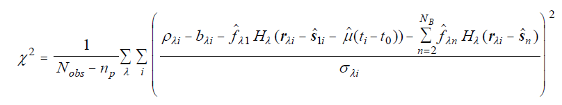 | Eq. 4 |
The inclusion of the 2-vector μ enlarges np by 2. The rest of the processing is the same as before except for the larger parameter space and the additional output source parameters for the motioncomponents and their associated uncertainties. Since actively deblended sources never take on the role of primary component of an ensemble, their motion is not estimated and will be null in the final products.
The uncertainty estimates for motion are obtained in a manner corresponding to the parameter uncertainty estimation of previous versions of WPHOT. The only difference is the inclusion of the motion terms in the model and chi-square. The Fisher information matrix G is computed, and the error covariance matrix γ expressing the parameter uncertainties is the inverse of G:
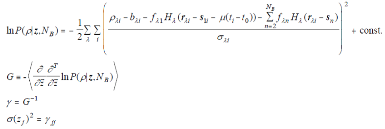 | Eq. 5 |
where ρ is the vector of all pixels used for the calculation, with Nobs elements, and z is the vector of all parameters being fit, with npelements. The G and γ matrices are therefore np×np in size. The components of the z vector are [s10, (fλ1 : λ=1 to Nλ, {sn , ( fλn : λ = 1 to Nλ )} : n = 2 to NB , μ].
The dependence of γ on μ is via the dependence of Hλ on s1, whose derivatives may take on positive, negative, or zero values, depending on where in the PSF a given pixel falls, and since the PSF models are numerical, not algebraic, and also since the total dependence involves a sum over all pixels used in the computation, how the new motion parameters affect the uncertainties of the fluxes is most readily investigated numerically rather than algebraically. Averages of the full error covariance matrix over thousands of typical sources revealed no significant correlation between motion errors and flux errors. Furthermore, any significant error correlation between motion and position at the reference epoch is removed by the use of the flux-weighted mean epoch as the reference epoch for the PM solution. As always, however, some motion-position error correlation is introduced by translating the position from the source-peculiar mean observation epoch to the AllWISE standard epoch of MJD 55400 via the motion rates multiplied by the difference in epochs.
V.3.b.ii.3. Gradient-Descent Algorithm
Section IV.4.c.iii of the Explanatory Supplement to the WISE All-Sky Data Release Products defines the figure of merit used to estimate point-source fluxes and position. This is summarized in section V.b.3.ii.1 above, and the addition of source motion is described in section V.b.3.ii.2 above.
Both the stationary and the PM models are implemented in AllWISE. In each case the best solution is taken to be that which minimizes the model's chi-square. Because the models are nonlinear in the parameters to be estimated, the solutions cannot be obtained in one step by matrix inversion, and an iterative method is required. As with all iterative methods for solving nonlinear systems, starting estimates are needed. The stationary solution is obtained first, with starting estimates provided by the MDET positions and the aperture fluxes derived from the measurements at that position. Then the PM solution begins at the stationary-solution positions with initial motion estimates of zero. From the starting estimates, improved estimates (i.e., which reduce chi-square) are sought via the gradient-descent method. That is, the gradient of chi-square in the parameter hyperspace is computed, and chi-square is evaluated at successive points in the negative direction of the gradient until a minimum is detected.
The stationary model parameter hyperspace is 6-dimensional in AllWISE for a single source, namely two position parameters (one per axis) and four fluxes. The PM model adds two motion parameters (one per axis) for the primary component of a passive-blend group. In passive-blend groups containing more sources than just the primary component, another six dimensions are added for each additional source in both models. Given estimates for the position(s), which are time-dependent for the primary component in the PM model, the fluxes can be computed directly from the frame data by fitting to the PSF template. This last step is a linear problem. Because of PSF uncertainty, the flux uncertainties do depend on the flux, which makes the problem nonlinear in principle, but whenever the model is evaluated, fluxes from a previous evaluation are used to compute the PSF component of uncertainty, starting with the initial aperture fluxes. Once new estimates of the fluxes are available, chi-square can be computed. So the problem becomes one of efficiently finding position and motion values for which the corresponding flux estimates minimize chi-square.
Since the stationary model is a subset of the PM model, we will focus on the latter, with the understanding that references to motion do not apply to the stationary model. The position and motion model parameters are represented formally by a vector denoted P, and the algorithmic description is the same for both models except for the length of the P vector. The search for the chi-square minimum is therefore confined to the position-motion space whose parameters are stored in a P vector of length 2N+2, where N is the number of sources in the blend group, each with two position parameters, and the primary component with two motion parameters in the PM model. In the notation of section V.3.b.ii.2, the components of the P vector are the N s vectors with the μ vector as the last two elements.
The location of the chi-square minimum in the P space is found by searching for it at discrete locations. A step size S of length equal to 1% of the minimum frame pixel size is used, which amounts to about 0.0275 arcsec for position parameters and 0.0275 arcsec/year for motion parameters. The search involves taking the following actions from each "base location", where the first base location is at the P vector corresponding to the MDET position(s) for the stationary model, and corresponding to the stationary solution and zero motion for the PM model. Each selection of a base location begins one "iteration" in the search.We denote the base location as P0, the gradient of chi-square at a base location is g, and the nth trial point in the iteration is Pn, at which point the value of chi-square is Cn.
- g and C0 are calculated at the base location, and the gradient magnitude |g| is computed; if |g| is zero, the minimum has been found, and the search ends, otherwise the following actions are taken.
- A step ΔP = S/|g| is computed, the step counter n is initialized at 0, and then the following operations are performed:
- The components of the Pn+1 vector are computed: Pn+1(i) = Pn(i) - ΔP g(i) for all 2N+2 components i of the vectors;
- Cn+1 is evaluated at Pn+1;
- if Cn+1 > Cn or n+1 ≥ nmax (where nmax is 100 for the stationary solution and 250 for the PM solution), then terminate this part of the search, otherwise increment n and resume at step B1 above.
- Take one step back: Pn(i) = Pn+1(i) + ΔP g(i), increment the iteration counter.
- Compute ΔC = 2|C0 - Cn | and Cmin = 10-3|C0 + Cn + 10-10|.
- If Cn ≥ C0 then go to step F, otherwise if ((ΔC ≤ Cmin) or (number of iterations is 100)) then end the search with Pn, otherwise P0 ⇐ Pn, go back to step A.
- If (ΔC ≤ 0.01Cmin) or (number of iterations is 100) then end the search with Pn, otherwise continue.
- The search has overshot the solution; P0 ⇐ Pn, S ⇐ S/2; go back to step A.
Subtracting ΔP g(i) from Pn(i) in step B.1 causes stepping in the negative gradient direction, hence the direction in which chi-square gets smaller. The normalization of the step by the magnitude of the gradient has the effect of multiplying a unit vector U by the step size S, where U = g/|g|.
In the stationary solution, when there is only one source in the passive-blend group, the P vector has a length N = 2, and so the U vector lies in this plane, and step B.1 moves the P vector a radial distance of exactly S, whose initial value is 0.0275 arcsec. If the chi-square minimum is found before reaching step G, then it will be found at some radial distance from the MDET position that is an integral multiple of 0.0275 arcsec. This quantizes the solution relative to the initial position estimate, but this is generally not visible because the quantized offsets are relative to a different MDET source in each case. Nevertheless, plots of the P vector components for a large collection of sources show a strong tendency to be quantized in circles of radius 0.0275k, where k is an integer. Each time step G is reached, if at all, the quantization length is cut in half. Step G is reached only when a search step overshoots the solution by a significant amount, indicating a need for a finer step size and a new evaluation of the gradient. The high degree of quantization at the initial step size of 0.0275 indicates that most sources never reach step G.
When the stationary solution is obtained for a blend group containing more than the primary source, then in general all sources have significantly non-zero components of U on their position axes, and no individual source gets a radial step of 0.0275 arcsec, so no quantization is conspicuous. The same is true if step G is reached, because the step size is cut in half one or more times. If one knows to look, some quantization can occasionally be detected at 0.0275k/2m, where m is the number of activations of step G, but it usually does not call attention to itself.
The sharing of the U vector's components over all P axes is usually not the case with the motion parameters of the PM solution, because very frequently the position parameters used as initial estimates are converged for all practical purposes, leaving only the motion plane to receive almost all of the gradient unit vector, hence initial search steps of 0.0275 arcsec/year. Since one finds what one is seeking only where one looks for it, the chi-square minimum is found in such quantized locations of the motion space, as seen in Figure 1 below, a plot for a typical tile.
 |
| Figure 1 - A plot of RA and Dec motion measurements for detections in a typical Tile that illustrates the motion quantization. |
This manifestation of quantization is the one in which the phenomenon was discovered, after which the cause for quantization in stationary position and PM motion was reconstructed. Since the PM solution has motion parameters only for the primary source in a blend group, the presence of other sources in that group does not significantly disturb the motion quantization in most cases.
V.3.b.ii.4. Effect of Noise on the Motion Solution
Chi-square minimization is one of the most powerful methods for estimating model parameters from measurements subject to noise, but the mere presence of noise in the measurements virtually assures the presence of some error in the estimated parameters. This can be quite noticeable when the correct value of a parameter is essentially zero (i.e., extremely small), since any non-zero result is purely the product of noise.
When the parameter being estimated is source motion on the sky, the fact that most sources detectable by WISE have true motions over the observational time span below the WISE spatial resolution leads inevitably to an abundance of pure-noise estimates. In most cases, these noise-produced motions are typically of the order of the motion uncertainty, i.e., not statistically significant. For faint low-S/N sources, however, it sometimes happens that chi-square can be reduced by fitting photometric noise variations in the single-frame observations. It is actually rather rare not to be able to achieve some chi-square reduction by finding some spurious motion that seems partially to explain the photometric variations that are actually just due to noise. This is a common hazard of nonlinear models with a large number of fitting parameters.
In some cases, this stretching of the truth proceeds to rather large motion estimates that may appear significant relative to their uncertainties, because the formal uncertainties have nothing to do with goodness-of-fit (only chi-square can indicate that, and it can fail in these cases because it is what is specifically being minimized), they depend only on the prior uncertainties due to measurement noise, which need not be particularly large to remain compatible with large flat regions in the chi-square hyperspace.
Even chi-square can be unreliable when some implausibly large motion allows the model to be fit better than the stationary model, but the formal motion uncertainties can definitely be misleading, because what they indicate is not goodness-of-fit but rather the uncertainty in whether the model parameters are the best possible compared to other values of the model parameters. In other words, a linear fit to low-noise parabolic data may have very small parameter uncertainties despite a terrible chi-square goodness-of-fit value, because the parameter uncertainties reflect only how good that linear fit is compared to all other possible linear fits. When the model doesn't fit the data, the parameter uncertainties have little to do with anything, and when photometric noise fluctuations prevent a source's true non-moving nature from being obvious, very large spurious motion estimates can result. Chi-square, having been minimized, is more a metric of how the measurements don't rule out large motion than an argument that the motion must be large.
These situations do have a rather characteristic behavior in the PM solution. Because the chi-square hypersurface has no crystal-clear minimum, the search for a minimum over the noisy terrain (see section V.3.b.ii.3 above) can drift like a feather in the wind. But the gradient-descent algorithm has arbitrary surrender points when it seems that it is getting nowhere, and one of these is when it runs off the end of the current iteration's maximum number of steps. This corresponds to the algorithm step B.3 in the previous section; the PM solution uses nmax = 250, and that many steps of size 0.0275 arcsec/yr amounts to 6.875, which is where subsequent steps in the algorithm decide to punt. Thus there is a "pile-up" of motion estimates at or near 6.875 arcsec/yr, and these should essentially all be considered pure-noise solutions.
Figure 2 shows this conspicuous ring for a typical tile. The quantization shown in Figure 1 in section V.3.b.ii.3 is also present but cannot be resolved at this scale. The use of nmax = 250 in the PM solution was chosen specifically to force this "pile-up" to occur at an implausibly large radial-motion value.
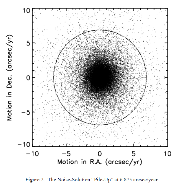 |
| Figure 2 - The Noise-Solution "Pile-Up" at 6.875 arcsec/year |
Thus there is a "pile-up" of motion estimates at or near 6.875 arcsec/yr, and these should essentially all be considered pure-noise solutions.
Last update: 19 November 2013