 |
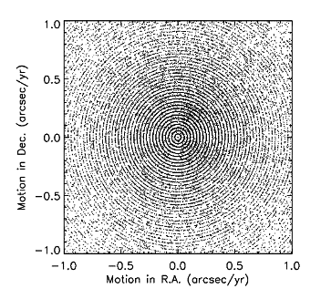
| Figure 2 - A plot for a typical tile. |


Section IV.4.c.iii of the Explanatory Supplement to the WISE All-Sky Data Release Products defines the figure of merit used to estimate point-source fluxes and position. This is summarized in section V.b.3.ii.1 above, and the addition of source motion is described in section V.b.3.ii.2 above.
Both the stationary and the PM models are implemented in AllWISE. In each case the best solution is taken to be that which minimizes the model's chi-square. Because the models are nonlinear in the parameters to be estimated, the solutions cannot be obtained in one step by matrix inversion, and an iterative method is required. As with all iterative methods for solving nonlinear systems, starting estimates are needed. The stationary solution is obtained first, with starting estimates provided by the MDET positions and the aperture fluxes derived from the measurements at that position. Then the PM solution begins at the stationary-solution positions with initial motion estimates of zero. From the starting estimates, improved estimates (i.e., which reduce chi-square) are sought via the gradient-descent method. That is, the gradient of chi-square in the parameter hyperspace is computed, and chi-square is evaluated at successive points in the negative direction of the gradient until a minimum is detected.
The stationary model parameter hyperspace is 6-dimensional in AllWISE for a single source, namely two position parameters (one per axis) and four fluxes. The PM model adds two motion parameters (one per axis) for the primary component of a passive-blend group. In passive-blend groups containing more sources than just the primary component, another six dimensions are added for each additional source in both models. Given estimates for the position(s), which are time-dependent for the primary component in the PM model, the fluxes can be computed directly from the frame data by fitting to the PSF template. This last step is a linear problem. Because of PSF uncertainty, the flux uncertainties do depend on the flux, which makes the problem nonlinear in principle, but whenever the model is evaluated, fluxes from a previous evaluation are used to compute the PSF component of uncertainty, starting with the initial aperture fluxes. Once new estimates of the fluxes are available, chi-square can be computed. So the problem becomes one of efficiently finding position and motion values for which the corresponding flux estimates minimize chi-square.
Since the stationary model is a subset of the PM model, we will focus on the latter, with the understanding that references to motion do not apply to the stationary model. The position and motion model parameters are represented formally by a vector denoted P, and the algorithmic description is the same for both models except for the length of the P vector. The search for the chi-square minimum is therefore confined to the position-motion space whose parameters are stored in a P vector of length 2N+2, where N is the number of sources in the blend group, each with two position parameters, and the primary component with two motion parameters in the PM model. In the notation of section V.3.b.ii.2, the components of the P vector are the N s vectors with the μ vector as the last two elements.
The location of the chi-square minimum in the P space is found by searching for it at discrete locations. A step size S of length equal to 1% of the minimum frame pixel size is used, which amounts to about 0.0275 arcsec for position parameters and 0.0275 arcsec/year for motion parameters. The search involves taking the following actions from each "base location", where the first base location is at the P vector corresponding to the MDET position(s) for the stationary model, and corresponding to the stationary solution and zero motion for the PM model. Each selection of a base location begins one "iteration" in the search.We denote the base location as P0, the gradient of chi-square at a base location is g, and the nth trial point in the iteration is Pn, at which point the value of chi-square is Cn.
- g and C0 are calculated at the base location, and the gradient magnitude |g| is computed; if |g| is zero, the minimum has been found, and the search ends, otherwise the following actions are taken.
- A step ΔP = S/|g| is computed, the step counter n is initialized at 0, and then the following operations are performed:
- The components of the Pn+1 vector are computed: Pn+1(i) = Pn(i) - ΔP g(i) for all 2N+2 components i of the vectors;
- Cn+1 is evaluated at Pn+1;
- if Cn+1 > Cn or n+1 ≥ nmax (where nmax is 100 for the stationary solution and 250 for the PM solution), then terminate this part of the search, otherwise increment n and resume at step B1 above.
- Take one step back: Pn(i) = Pn+1(i) + ΔP g(i), increment the iteration counter.
- Compute ΔC = 2|C0 - Cn | and Cmin = 10-3|C0 + Cn + 10-10|.
- If Cn ≥ C0 then go to step F, otherwise if ((ΔC ≤ Cmin) or (number of iterations is 100)) then end the search with Pn, otherwise P0 ⇐ Pn, go back to step A.
- If (ΔC ≤ 0.01Cmin) or (number of iterations is 100) then end the search with Pn, otherwise continue.
- The search has overshot the solution; P0 ⇐ Pn, S ⇐ S/2; go back to step A.
Subtracting ΔP g(i) from Pn(i) in step B.1 causes stepping in the negative gradient direction, hence the direction in which chi-square gets smaller. The normalization of the step by the magnitude of the gradient has the effect of multiplying a unit vector U by the step size S, where U = g/|g|.
In the stationary solution, when there is only one source in the passive-blend group, the P vector has a length N = 2, and so the U vector lies in this plane, and step B.1 moves the P vector a radial distance of exactly S, whose initial value is 0.0275 arcsec. If the chi-square minimum is found before reaching step G, then it will be found at some radial distance from the MDET position that is an integral multiple of 0.0275 arcsec. This quantizes the solution relative to the initial position estimate, but this is generally not visible because the quantized offsets are relative to a different MDET source in each case. Nevertheless, plots of the P vector components for a large collection of sources show a strong tendency to be quantized in circles of radius 0.0275k, where k is an integer. Each time step G is reached, if at all, the quantization length is cut in half. Step G is reached only when a search step overshoots the solution by a significant amount, indicating a need for a finer step size and a new evaluation of the gradient. The high degree of quantization at the initial step size of 0.0275 indicates that most sources never reach step G.
When the stationary solution is obtained for a blend group containing more than the primary source, then in general all sources have significantly non-zero components of U on their position axes, and no individual source gets a radial step of 0.0275 arcsec, so no quantization is conspicuous. The same is true if step G is reached, because the step size is cut in half one or more times. If one knows to look, some quantization can occasionally be detected at 0.0275k/2m, where m is the number of activations of step G, but it usually does not call attention to itself.
The sharing of the U vectors components over all P axes is usually not the case with the motion parameters of the PM solution, because very frequently the position parameters used as initial estimates are converged for all practical purposes, leaving only the motion plane to receive almost all of the gradient unit vector, hence initial search steps of 0.0275 arcsec/year. Since one finds what one is seeking only where one looks for it, the chi-square minimum is found in such quantized locations of the motion space, as seen in Figure 1 below, a plot for a typical tile.
 |
| Figure 2 - A plot for a typical tile. |
This manifestation of quantization is the one in which the phenomenon was discovered, after which the cause for quantization in stationary position and PM motion was reconstructed. Since the PM solution has motion parameters only for the primary source in a blend group, the presence of other sources in that group does not significantly disturb the motion quantization in most cases.
Last update: 2013 October 28