II. AllWISE Source Catalog and Reject Table

II.4. Completeness and Reliability

II.4.a. Catalog Completeness

Contents

II.4.a.i. Summary

Completeness is the quantity that describes the fraction of real sources that are detected. Put another way, it's the probability that a source is detected given that a source exists to be detected. In formal statistics completeness is closely related to what is called a "type II error," or a false positive. Completeness is therefore an important metric of a catalog's performance and an essential tool for working with data near the limit of a survey's sensitivity.

The AllWISE Source Catalog does not have any completeness level it is formally required to meet. We show herein that AllWISE meets and surpasses the requirements imposed on the WISE All–Sky data release, with the possible exception of sources affected by the W1 saturation problem near the beginning of the 3–band cryo stage of the mission, and even exceeds the completeness of the All–Sky at the same coverage most over most of the sky in the short wavelength band (W1) due to the reduction of the background over–subtraction issue.

In the process of examining completeness we found a deficit in high snr sources for W1. Details of the cause of the problem are in Section V.1.b.iii.. Figure 1 shows that the problem is well isolated in two stripes of ecliptic longitude. We therefore split the analysis of completeness for AllWISE by ecliptic longitude into the High W1sat stripes ($45°<\lambda <59°$ or $229°<\lambda <243°$), and the Main Sample outside of those stripes.

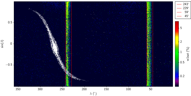Figure 1 – Cylindrical equal area projection of AllWISE sources satisfying $15.0\le \mathrm{w1mpro}<15.05$ on an ecliptic grid. The color of the points encodes the fraction of W1 pixels in the source that were saturated. Because the sources are faint, 15th magnitude, all of the saturated pixels are exogenous (eg: cosmic ray hits, contamination). The red vertical lines highlight the rough boundaries in ecliptic longitude that separate the stripes with high w1sat from the regions containing the main sample.

The approach we take in assessing completeness for AllWISE is very different than what was done for All–Sky. Like for assessing reliability, any assessment of completeness begins with the construction of a "truth list," a list of sources that WISE could detect and the fluxes WISE would measure for them. In order to be useful, the truth list must be both more sensitive than WISE and highly reliable; unreliability in the truth list looks like false incompleteness, just as incompleteness in the truth list can falsely lower measured reliability. For Allsky, we produced truth lists using external data from Spitzer/IRAC and internal lists based on artificially decimating the coverage of tiles, using the source list from the deepest versions of the tiles as the truth lists, as described in Section VI.5.b. of the WISE All–Sky Explanatory Supplement. The former truth sets are not available on a very large area of the sky to sufficient depth, and we did not have the resources to do the latter. We therefore leveraged the list of stellar models based on data from Sloan Digital Sky Survey, data release 9, (SDSSdr9) and Two Micron All Sky Survey (2MASS) presented by Lake et al. at winter AAS 2013 to evaluate the completeness of WISE's two short wavelength bands, W1 and W2, the ones with significantly increased depth in AllWISE. For the long wavelength bands, W3 and W4, it is safe to assume that the completeness is identical to WISE All–Sky because the underlying data content of the frames is the same. Time permitting, we will assess the completeness W3 and W4 at a later date using a less detailed analysis, boot strapping a truth list of color selected stars from 2MASS, W1, and W2. Focusing on a single source type, ordinary stars, forces us to assess completeness based on whether the source meets the selection criteria for the particular band being assessed, not the catalog. The advantages of this approach are: it permits a detailed assessment of how coverage affects completeness over a large area, and it makes it possible to calculate the completeness of sub–populations with unusual colors. The disadvantage of this approach is that it doesn't permit a meaningful assessment of the global completeness of the catalog. For that reason, the summary of AllWISE's completeness in Table 1 includes on fluxes for which AllWISE achieves 95% completeness based on the performance of a single band in the given range of coverages. For any source which exceeds these limits in any band, that isn't lost to contamination or confusion, AllWISE will be at least 95% complete before applying any Eddington bias correction.

II.4.a.ii. Comparison with SDSS Selected Stars

In order to maximize the reliability of the truth list, we required that all SDSSdr9 selected targets: exhibit stellar morphology, be high signal to noise in all 5 SDSS filters, have no SDSSdr9 detected neighbors within 15 arcseconds, be at high galactic latitude ($b\ge 30°$), and have high quality photometry. Where high quality 2MASS photometry was available it was used to constrain the stellar models, too. We then fit the data using the ATLAS 9 grid of stellar atmosphere models of Kurucz (1993) (only those of the form GRIDPnn or GRIDMnn), subject to interstellar dust extinction using the model of Cardelli et al. 1989 (doi:10.1086/167900, assuming $R_{\nu }=3.1$). Selecting for only those sources that were well modelled left 1,346,467 targets, shown in an ecliptic projection of the sky in Figure 2. Full details are in the Stellar Modeling Details section.

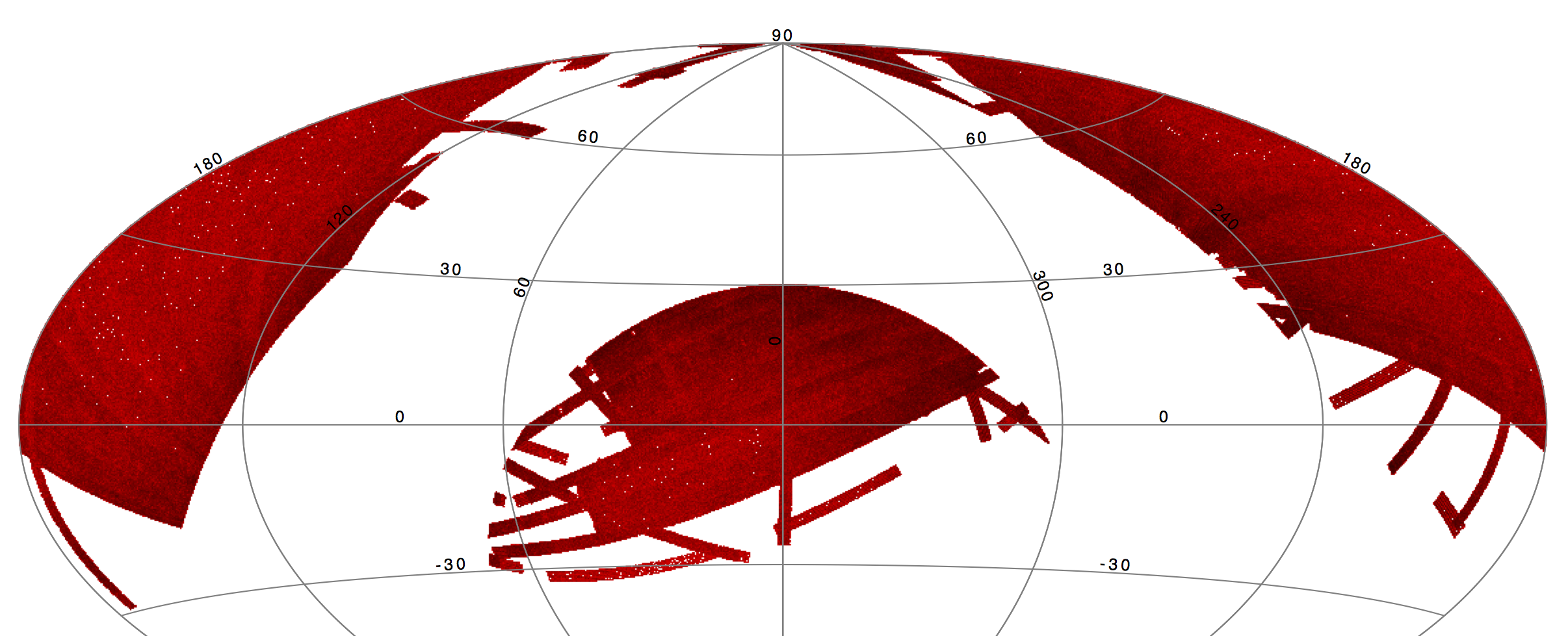Figure 2 – Aitoff projection of well modelled stars on the Ecliptic coordinate grid.

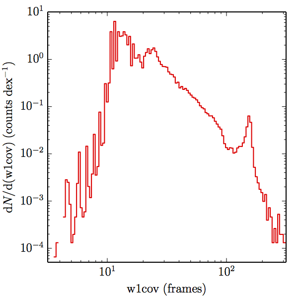
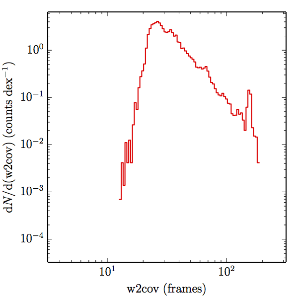
Of the 1.3 million stars in the global sample, the relative uncertainty of the W1 prediction is $\le 0.2$ for 974,553 of them, and likewise for 953,907 of them in W2. There are not enough well modelled stars bright enough in W3 to measure completeness, and none in W4. Dividing the samples into main and high w1sat gives: 880,106 and 94,447 in W1, and 861,508 and 92,399 in W2, each respectively. The frame coverages probed by the W1 and W2 samples are shown in Figure 3 for both AllWISE and All–Sky. The extent to which the histograms in Figure 3 differ from those in (link to coverage section) measures how accurately the overall coverage measures of completeness represents the catalog.

Band	AllWISE Main (1)	AllWISE High W1sat (2)	WISE All–Sky (3)
W1 (a)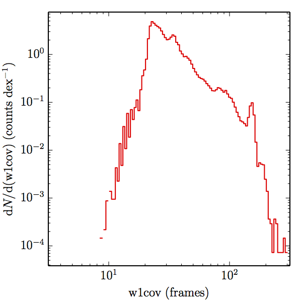
W2 (b)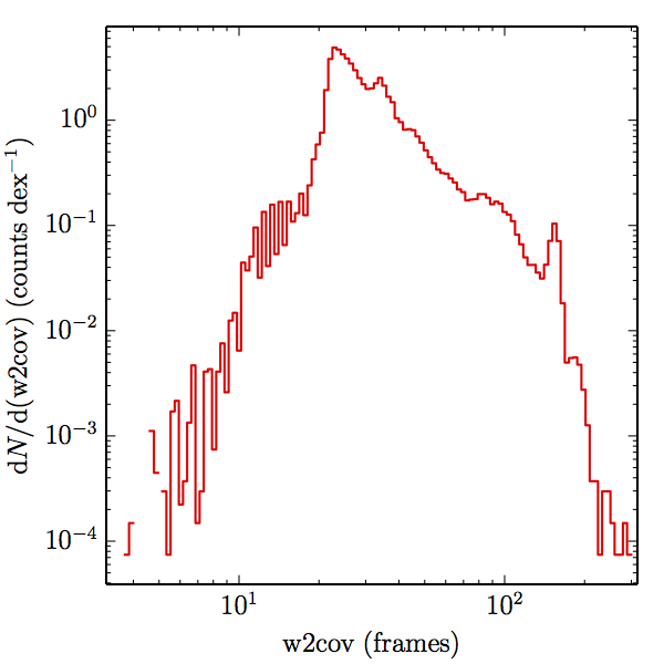
Figure 3 – Histograms of coverages probed by the SDSSdr9 selected stellar samples, as estimated by the nearest source in the AllWISE combined catalog (the union of the AllWISE catalog and reject table that is marked with use_src = 1). The first row (a) contains the W1 samples, and the second (b) the W2 samples. The first column (1) contains the AllWISE Main samples, the second (2) the AllWISE High W1sat samples, and the third (3) the All–Sky samples.

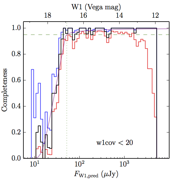
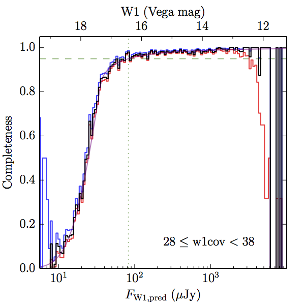
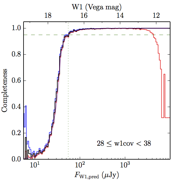
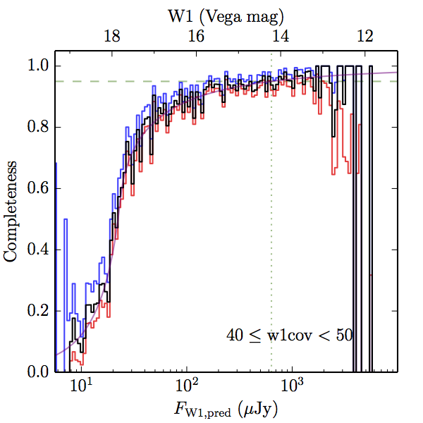
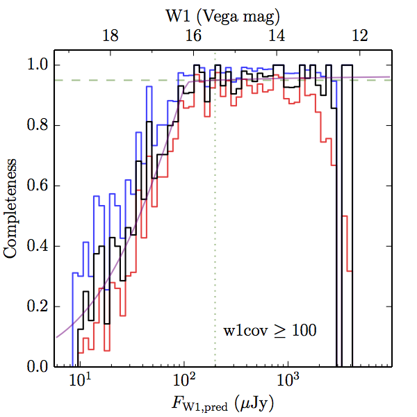
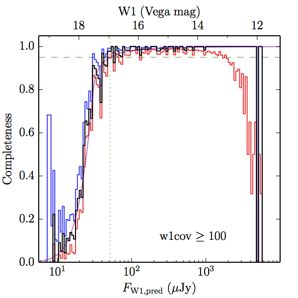
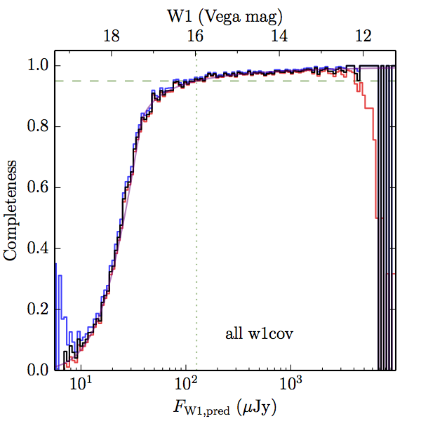
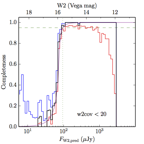
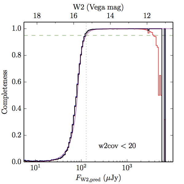
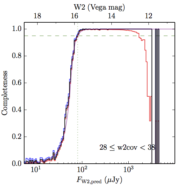
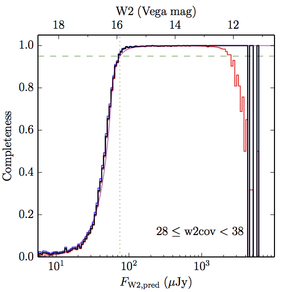
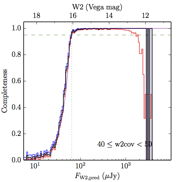
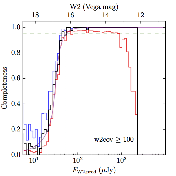
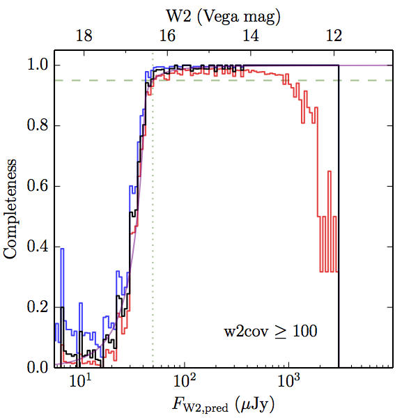
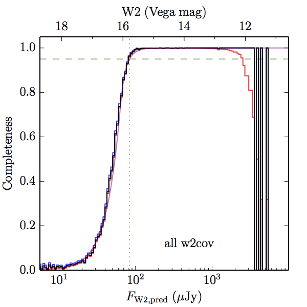
We searched for the truth list in the AllWISE combined catalog (the union of the AllWISE catalog and reject table) requiring that use_src = 1. We then repeatedly searched for unmatched sources, expanding the search radius for until there was a nearest neighbor of every source in the truth list. It is the coverage of that nearest neighbor that served as a proxy for the coverage of the source. This means that undetected sources have a slight bias toward higher coverages, but the effect should be small. A source was considered detected if the nearest AllWISE source was $\le 3$ arcseconds from the truth source and the WISE source satisfied the catalog selection criteria described in section (link) for the individual band being measured. Because using model stars is so radically different from the approach taken for All–Sky, we performed this task for WISE All–Sky, too. The detected sources and truth sources were then binned into histograms. Dividing the detected sources histogram by the truth list histogram gives a histogrammed "differential" completeness. The plots of completeness for different coverage cuts are in Figure 4 for W1 and Figure 5 for W2. Table 2 contains a list of the fluxes at which the plots in Figures 4 and 5 achieve 95% completeness.

$\mathrm{w1cov}$	AllWISE Main (1)	AllWISE High W1sat (2)	WISE All–Sky (3)
< 20 (a)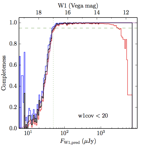
28–38 (b)
40–50 (c)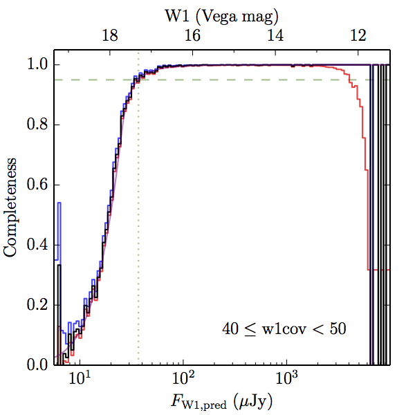
≥ 100 (d)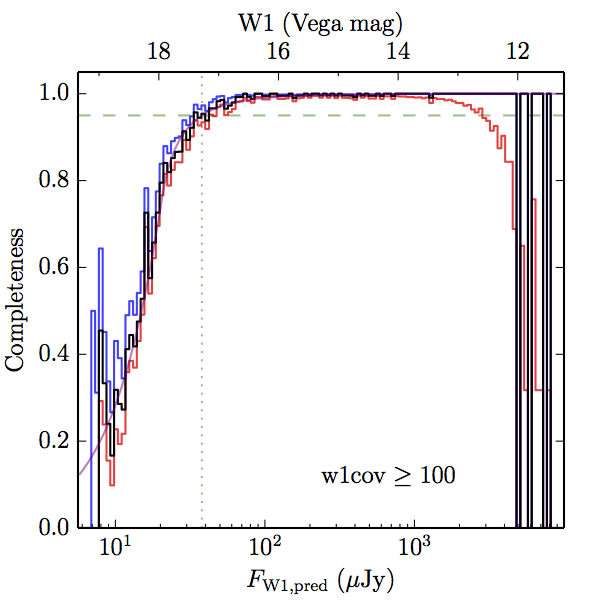
any (e)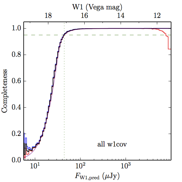
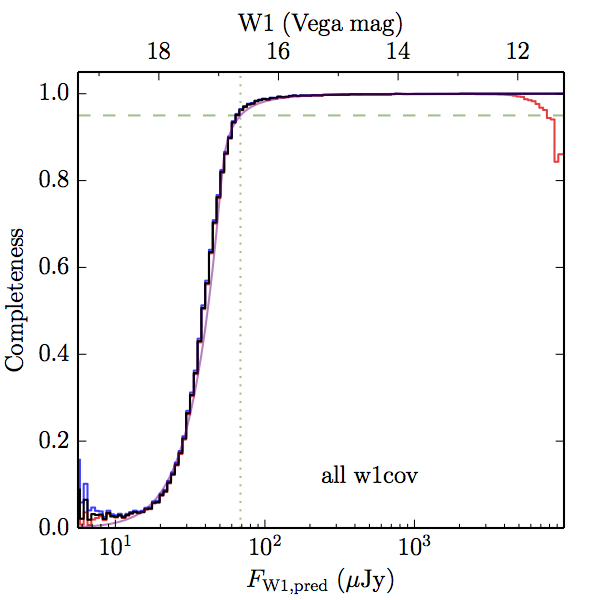Figure 4 – Completeness in W1 plotted versus predicted flux in WISE W1. The rows are different coverage ranges, and the columns are AllWISE Main (1), AllWISE High W1sat (2), and WISE All–Sky (3). The black line is the measured completeness, the blue and red lines bound the 1–sigma confidence band, the horizontal dashed line represents 95% completeness, the purple line is a best fit empirical model (see Section II.4.a.v.), and the vertical dotted line is where the model line hits 95% completeness. Note that the black line is set to zero when there are no truth sources in a given bin.

$\mathrm{w2cov}$	AllWISE Main (1)	AllWISE High W1sat (2)	WISE All–Sky (3)
< 20 (a)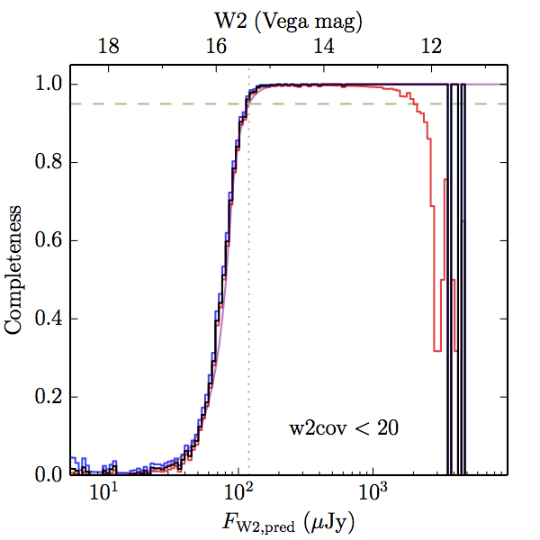
28–38 (b)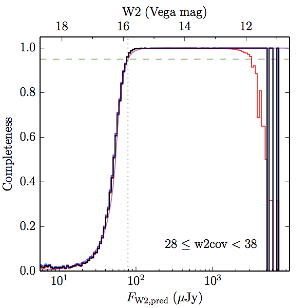
40–50 (c)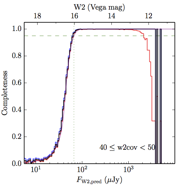
≥ 100 (d)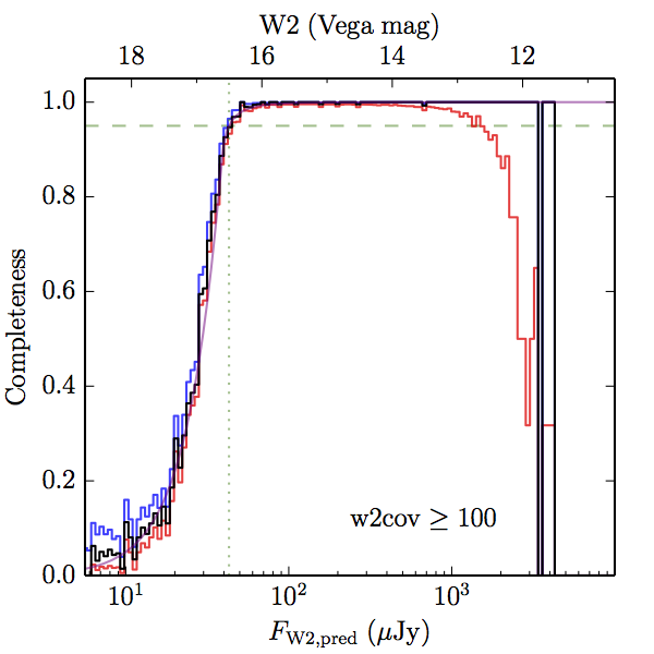
any (e)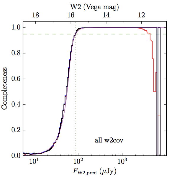
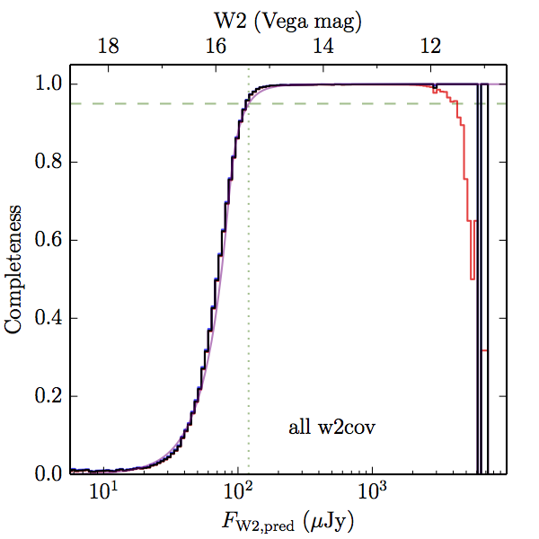Figure 5 – Completeness in W2 plotted versus predicted flux in WISE W2. The rows are different coverage ranges, and the columns are AllWISE Main (1), AllWISE High W1sat (2), and WISE All–Sky (3). The black line is the measured completeness, the blue and red lines bound the 1–sigma confidence band, the horizontal dashed line represents 95% completeness, the purple line is a best fit empirical model (see Section II.4.a.v.), and the vertical dotted line is where the model line hits 95% completeness. Note that the black line is set to zero when there are no truth sources in a given bin.

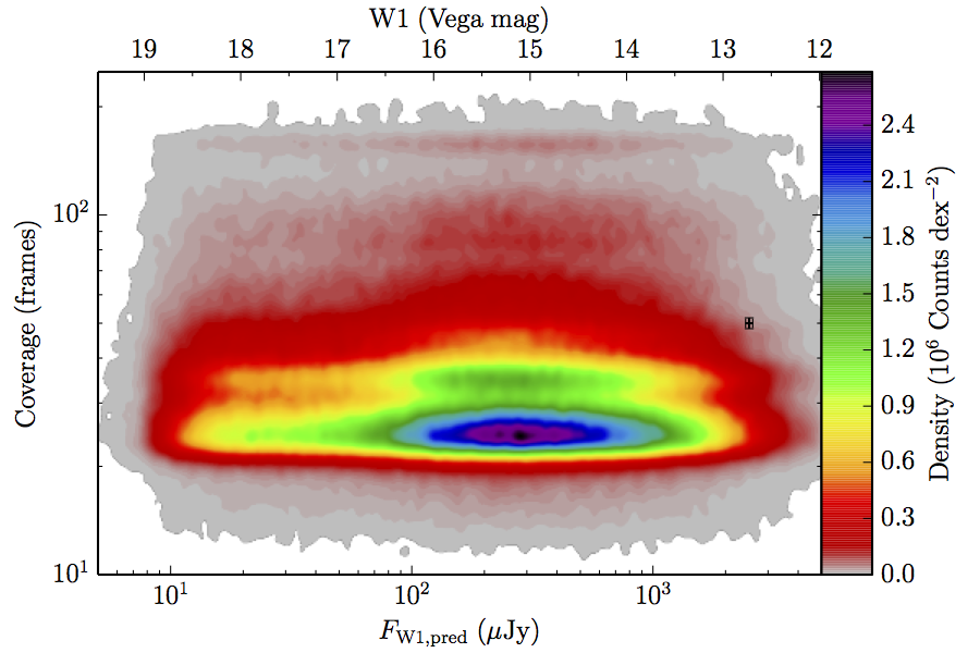
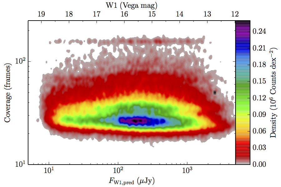
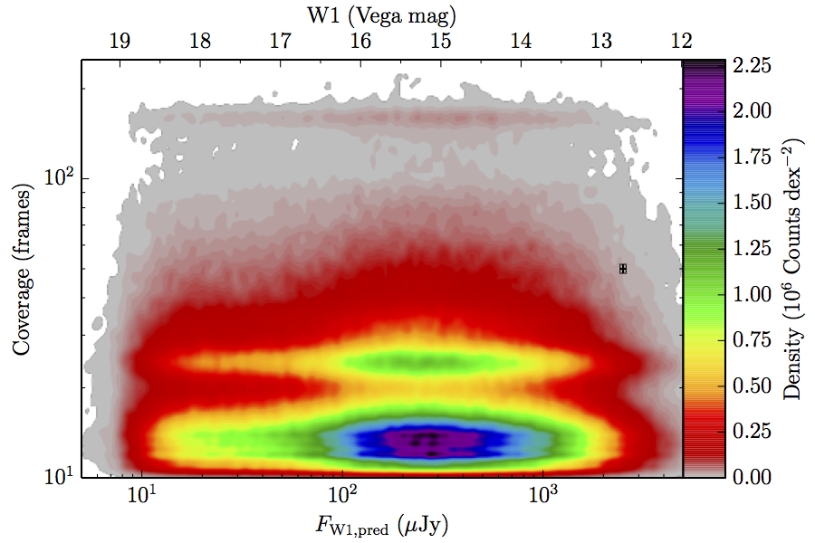
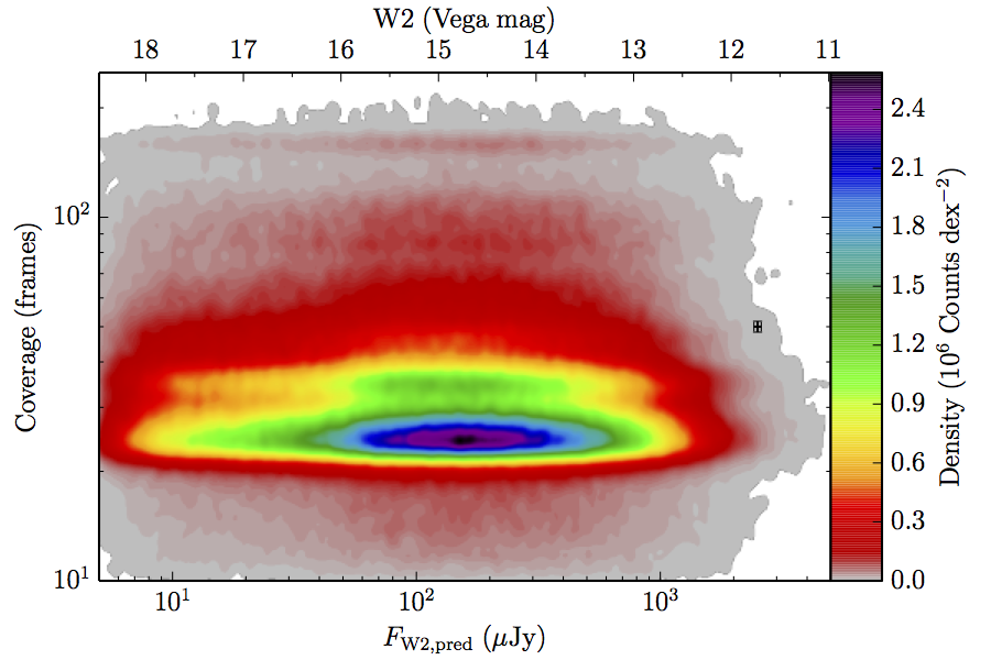
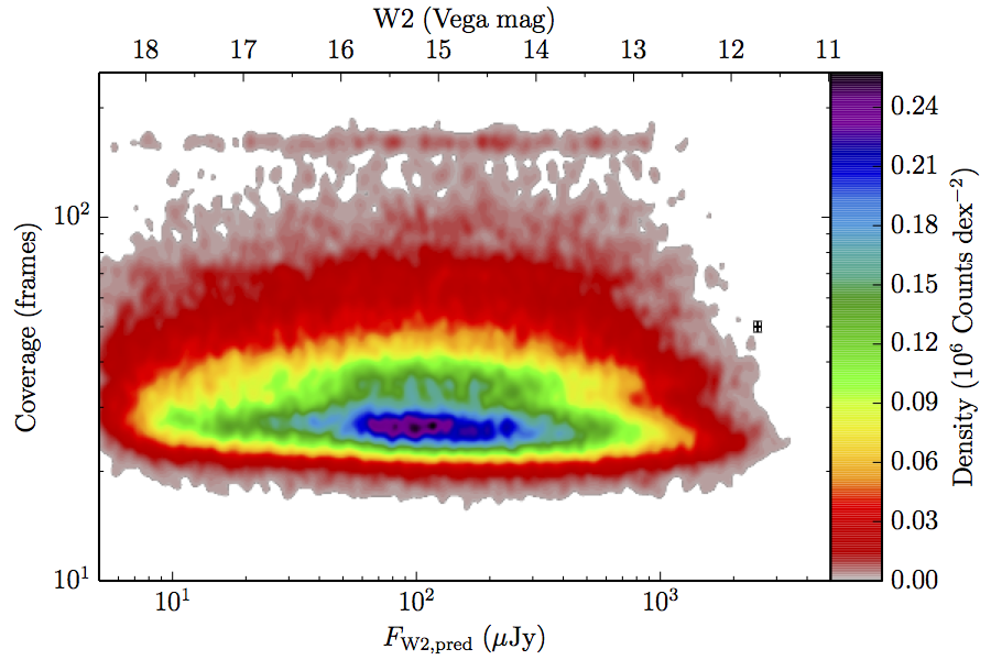
The large number of sources in our truth lists and large area on the sky permits an analysis that is far more finely binned in the coverage direction. Figure 6 contains source density in log coverage – log predicted flux space for the truth list and observed completeness in the same space. To produce the plots we binned the both the truth list and detected list on grids 1024 wide by 724 long. We then smoothed the both images by convolving with a Gaussian kernel with standard deviation 0.015 dex in both directions. The completeness image comes from dividing the smoothed detection image by the smoothed truth image. Finally, all pixels with a density lower than $4{\mathrm{e}}^{\mathrm{<mo>–</mo><mn>1</mn><mo>/</mo><mn>2</mn>}}/\left(2\mathrm{\pi }{\sigma }^2\right)\approx 1716{\mathrm{–2}}^{}$

Band	Sample	Completeness (1)	Truth Set Density (2)
W1	AllWISE Main (a)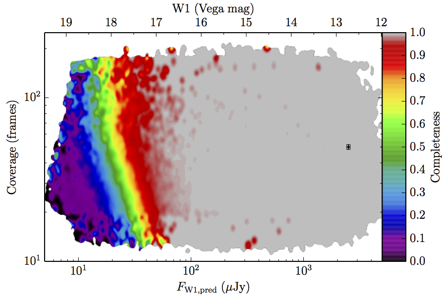
	AllWISE High W1sat (b)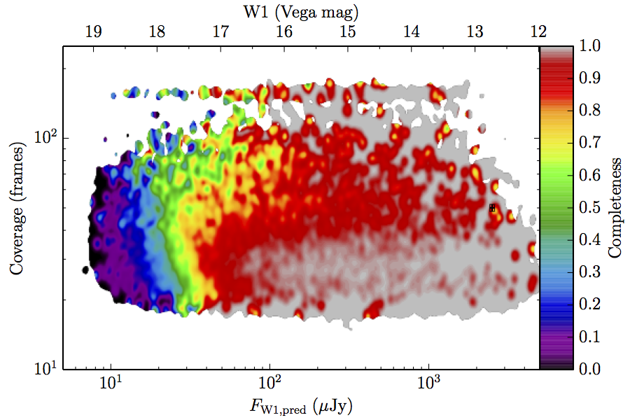
	WISE All–Sky (c)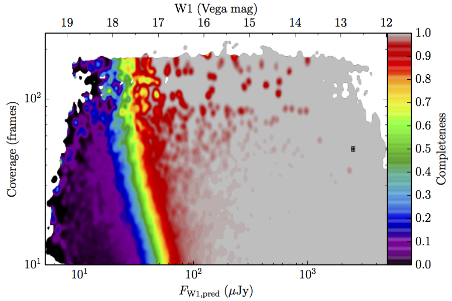
W2	AllWISE Main (d)
	AllWISE High W1sat (e)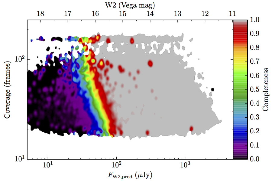
	WISE All–Sky (f)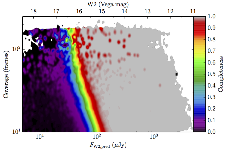
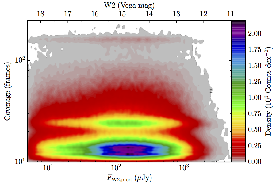Figure 6 – Completeness (column a) and sampling (truth set) density (column b) in log coverage – log flux space. Rows (a)–(c) contain plots about W1, and (d)–(f) contain plots about W2. Rows (a) and (d) are data from the AllWISE Main sample, (b) and (e) are from the AllWISE High W1sat sample, and (c) and (f) are from the WISE All–Sky sample. Each plot contains a point with error bars with the size of the error bars set to the 1–sigma scale of the smoothing.

II.4.a.iii. Comparison with Spitzer/IRAC

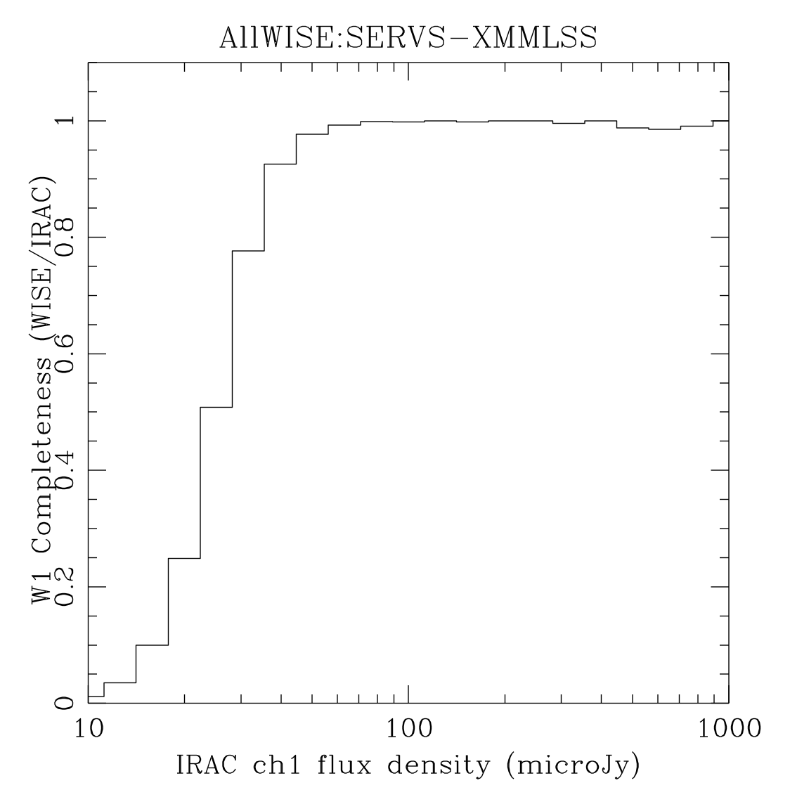
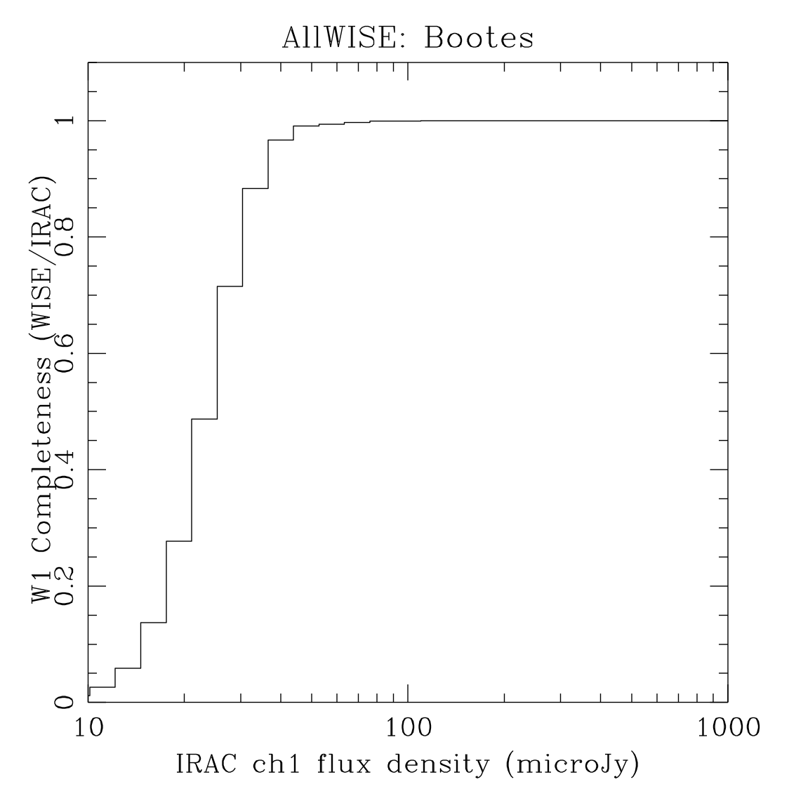
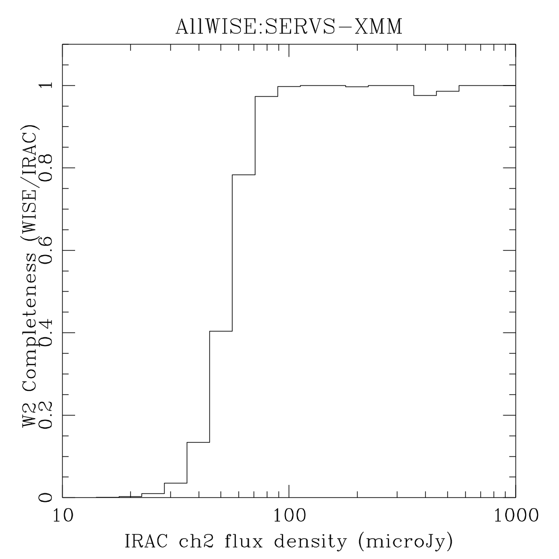
The planning for AllWISE included a comparison with external data sets generated by Spitzer/IRAC, similar to what was done for All–Sky. This more direct external test also has the advantage that it can also check the validity of the approach taken in Section II.4.a.ii.. The description for how the plots in Figure 7 were generated can be found in WISE All–Sky Explanatory Supplement Section VI.5.

The plots in Figure 7 are most directly comparable to the (b) rows of Figures 4 and 5 for the SERVS fields, and the (c) rows for Boötes. Table 3 contains estimates of the 95% completeness fluxes from linearly interpolating the plots in Figure 7. The figures therein are consistent with the coverage matching contents of Table 2.

	SERVS Lockman (1)	SERVS XMMLSS (2)	SDWFS Boötes (2)
W1/[3.6] (a)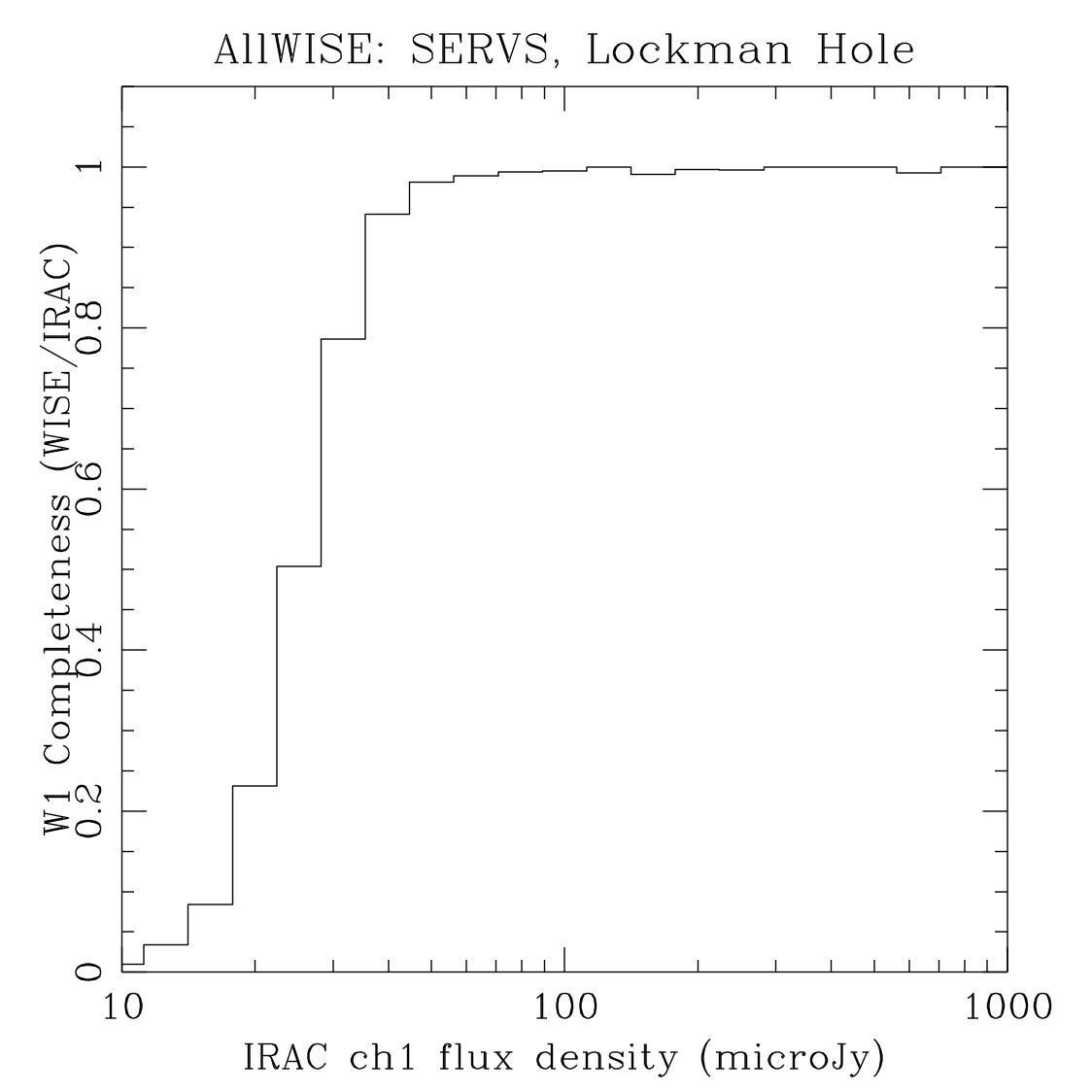
W2/[4.5] (b)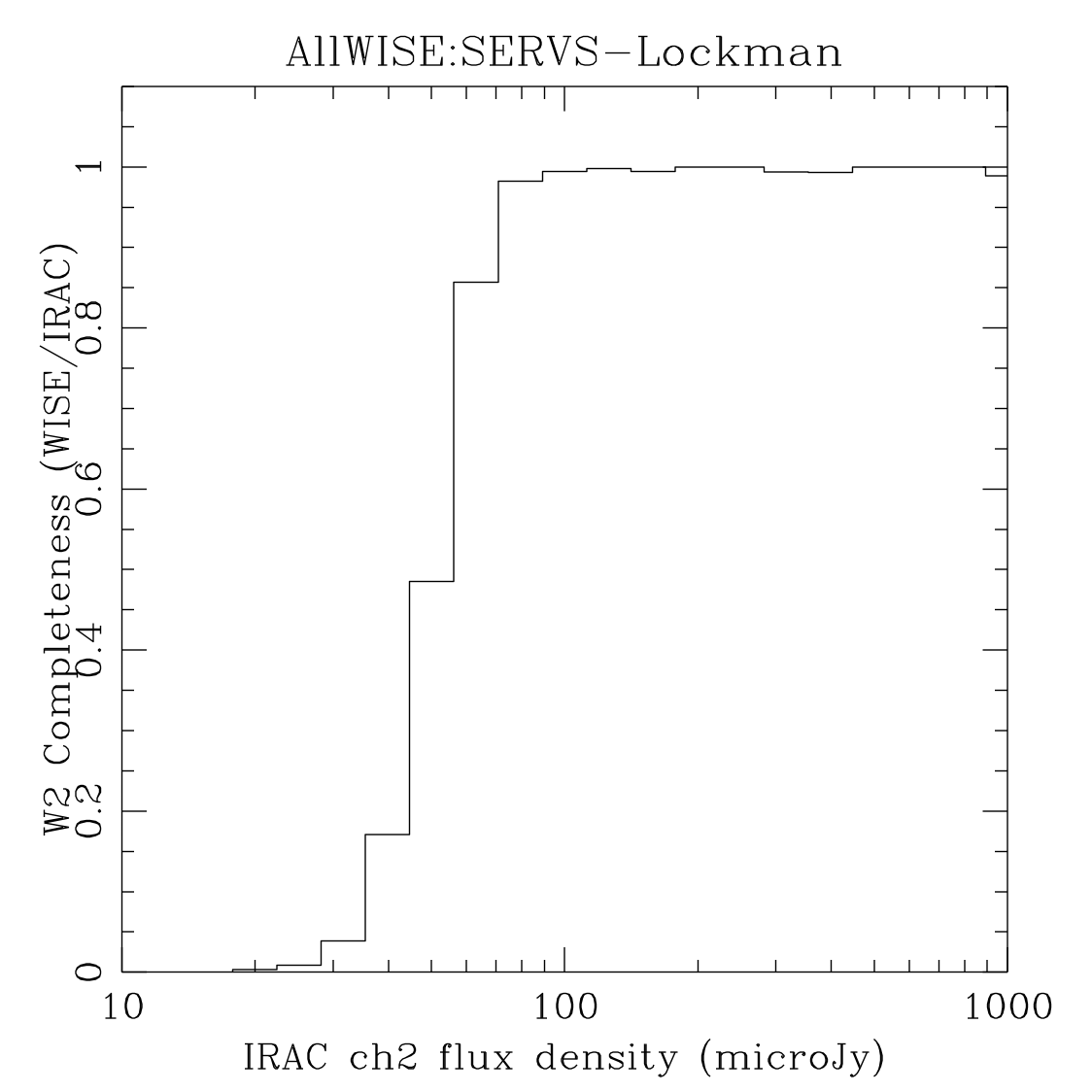
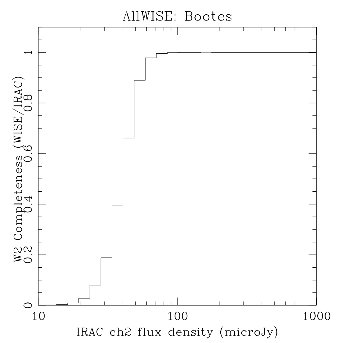Figure 7 – Completeness as measured by using catalogs produced from mosaics of Spitzer/IRAC images of the named fields as the truth set.

II.4.a.iv. Completeness in W3 and W4

The data content of AllWISE does not differ significantly from All–Sky for W3 and W4, so we did not put as much effort into measuring the completeness in these channels, and will be included in an addendum at a later date, time permitting.

II.4.a.v. Empirical Models of Completeness

The structure of the catalog selection criteria(link) makes the catalog functionally a union of 4 catalogs independently selected on each band. The initial source detection done by MDET(link) is based on a detection image that uses data from all 4 bands, so the independence of the catalogs is only approximate, but the high SNR cutoff for full catalog inclusion (SNR ≥ 5) mitigates this issue for assessing the catalog. Independence of selection means that in order for a source to be missed it must be missed by all 4 WISE bands. If the overall completeness is denoted $C$, and the completeness of band $i$ is $C_i$, then: $$C=1–\prod _{i=1}^4\left(1–C_i\right).\mathbf{\text{(II.4.a.v.1)}}$$ It is therefore possible to calculate the completeness of the catalog in terms of the completeness of the four WISE bands.

A full treatment of the $C_i$ would include a complicated treatment of confusion, the background, source flux, coverage, etc. We find that, as is can be seen in Figures 4 and 5, we have found that the following formula does a good job in approximating observed completeness for a fixed coverage: $$C\left(F\right)=\mathrm{CDF}\left({\log }_{10}\left(\frac{F}{F_{\mathrm{inflect}}}\right)\right),\mathbf{\text{(II.4.a.v.2)}}$$ where the definition of $\mathrm{CDF}\left(x\right)$, found in Equation II.4.a.v.3, is the integral of two Sérsic profiles with independent indicies and scale lengths, one for positive $x$ one for negative, continuously linked together. The main difference is that the Sérsic index is inverted. $F_{\mathrm{inflect}}$ is the flux at which the completeness undergoes a change in inflection.

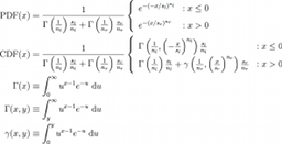Equations II.4.a.v.3 – Empirical equation used for fitting completeness.

Equation II.4.a.v.2 was fit to the data in Figures 4 and 5 using a maximum likelihood fit, where the likelihood was the product of the binomial distribution applied to each bin, $L_{\mathrm{bin}}=N_{\mathrm{true}}!/(n_{\det }![N_{\mathrm{true}}–n_{\det }]!)\times C_{\mathrm{model}}^{n_{\det }}{(1–C_{\mathrm{model}})}^{N_{\mathrm{true}}–n_{\det }}$. The fitting parameters that resulted from maximizing the likelihood for each of the plots in Figures 4 and 5 are in Table 4.

A simple addition to the model in Equation II.4.a.v.2 makes it suitable for modeling the images in Figure 6. The change is to make $F_{\mathrm{inflect}}$ a smoothly broken power law in coverage. Specifically: $$F_{\mathrm{inflect}}=F_0{\mathrm{cov}}_c^{\alpha }{\left({\left[\frac{\mathrm{cov}}{{\mathrm{cov}}_c}\right]}^{\alpha /s}+{\left[\frac{\mathrm{cov}}{{\mathrm{cov}}_c}\right]}^{\beta /s}\right)}^s,\mathbf{\text{(II.4.a.v.1)}}$$ where $\alpha ~\mathrm{–1}/2$ is the low coverage slope, $\beta ~0$ is the confusion limited slope, ${\mathrm{cov}}_c$ is the coverage where the completeness transitions to confusion limited scaling, $F_0$ is the constant of proportionality for asymptotically low coverage, and $s$ is the amount of smoothing in the power law transition.

The augmented model was fit to 2–dimensional histograms, unsmoothed, and binned more coarsely: 64 bins in log coverage, 138 in log flux. The fitting used the same likelihood as the 1–dimensional fits. The residuals of the smoothed image with respect to the fitted models are found in Figure 8, and the the parameters from those fits are found in Table 5.

Band	Subset	Residuals
W1	AllWISE Main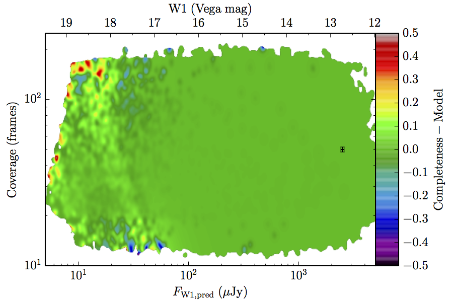
	AllWISE high w1sat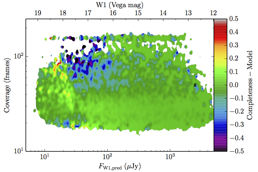
	WISE All–Sky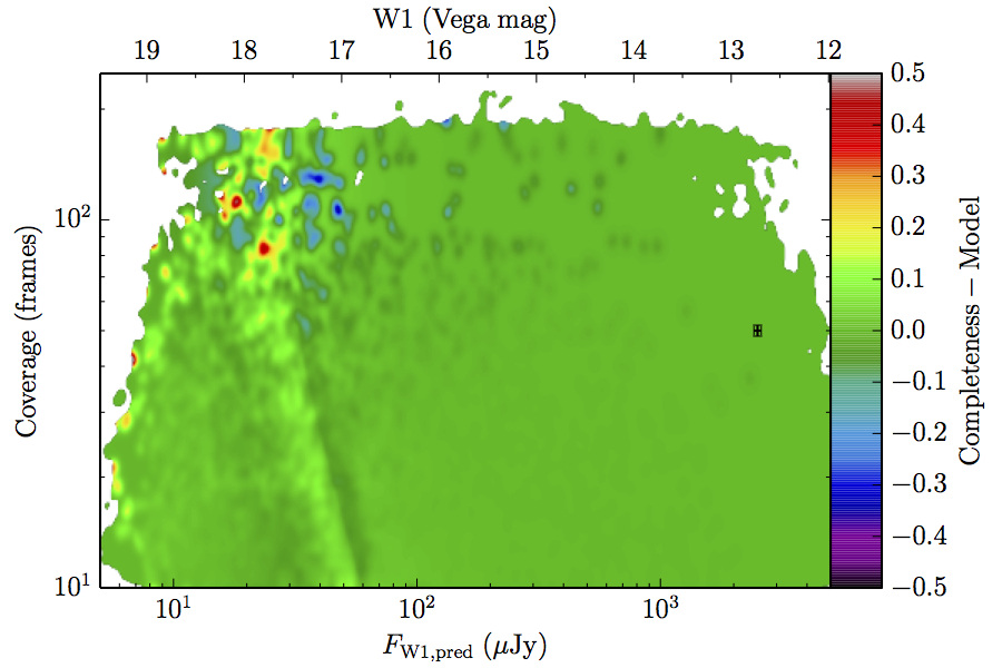
W2	AllWISE Main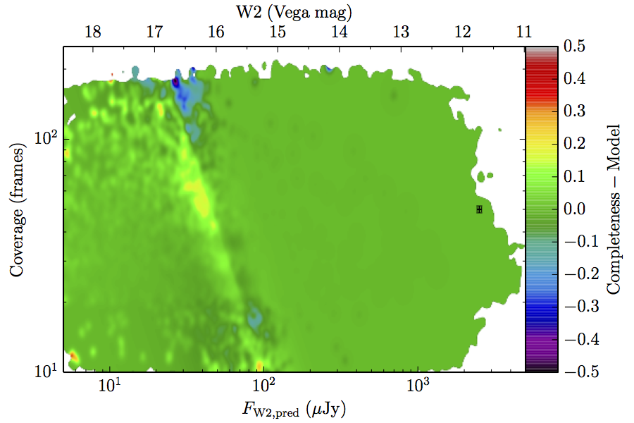
	AllWISE high w1sat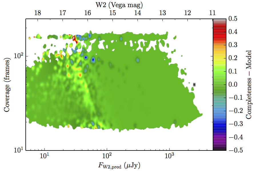
	WISE All–Sky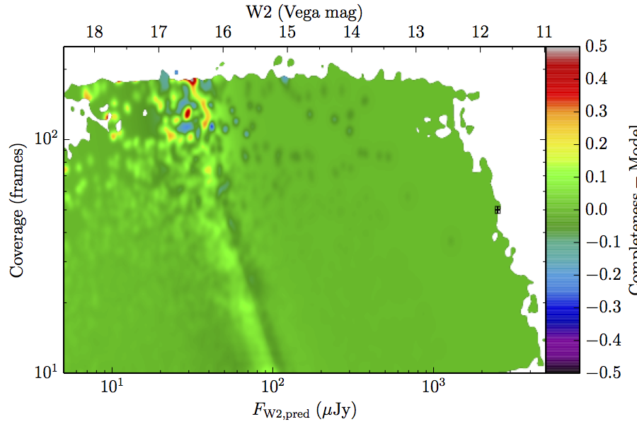
Figure 8 – Completeness residuals, observed in Column 1 of Figure 6 minus fitted model.

II.4.a.vi. Stellar Modeling Details

We retrieved the data using the SDSS CasJobs service to get data from SDSS Data Release 9, including the 2MASS data from the TwoMass Table on the same service. The data were required to satisfy all of the following:

• no SDSS detected primary neighbors within 15",
• high Galactic latitude ($\left|b\right|\ge 30°$),
• stellar morphology (type=6),
• brighter than 20.0 AB magnitude in SDSS $i$ filter ($\mathrm{psfFlux\_i}\ge 10.0$)
• high SNR in all 5 SDSS filters ( griz ≥ 5, u ≥ 3 ), and
• unblended, not a child, and far from the image edge ($\mathrm{flags}\&28=0$).

The fluxes from each 2MASS filter was used if the following flags were set: $\mathrm{ccFlag}=0$ and $\mathrm{blFlag}=1$. This process resulted in 4,412,967 candidate sources.

Combining the Kurucz stellar atmosphere grid with the Cardelli dust model yields 5 parameters to vary in the fitting of each star: effective temperature ($T_{\mathrm{eff}}$), metallicity (${\log }_{10}\left(Z\right)$), surface gravity (${\log }_{10}\left(g\right)$), distance to photosphere radius ratio ($D/R$), and color excess in $B–V$ ($E(B–V)$). These five parameters were varied to minimize ${\chi }^2$ , assuming Gaussian statistics in the fluxes. In principle, this means that there were zero degrees of freedom when no 2MASS photometry was available, but the model does not appear to actually cover enough 5–dimensional space to make this much of a problem. Indeed, Figure 9 shows that the same cuts in reduced ${\chi }^2$ work in straight ${\chi }^2$ when the formal number of degrees of freedom is zero. The full list of cuts is:

• typical badness of fit ($0.2\le {\chi }^2/\max \left(N_{\mathrm{df}},\; 1\right)\le 10$),
• cool stars were modeled poorly ($T_{\mathrm{eff}}>4750$ K),
• the minimizer (the L–BFGS–B minimizer in the scipy optimize package) must signal successful convergence,
• the optimal parameters must not be near the edges of the parameter search space,
• the eigenvalues of the Hessian matrix must all be positive definite,
• the nearest AllWISE source must not be associated with a 2MASS XSC source, and
• the nearest AllWISE source must be associated with at most one 2MASS point source.

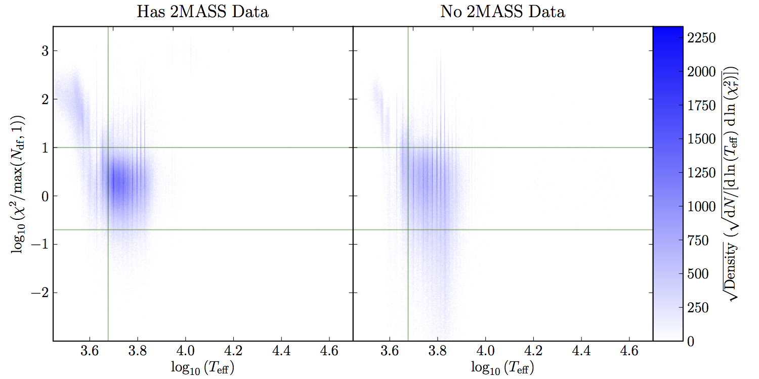Figure 9 – distribution of sources in ${\chi }^2$ – $T_{\mathrm{eff}}$ space. The green lines represent the cuts made to the data in this space: $0.2\le {\chi }^2/\max \left(N_{\mathrm{df}},\; 1\right)\le 10$, and $T_{\mathrm{eff}}>4750$ K. The vertical striping is due to the crude (non–continuous) linear interpolation used.

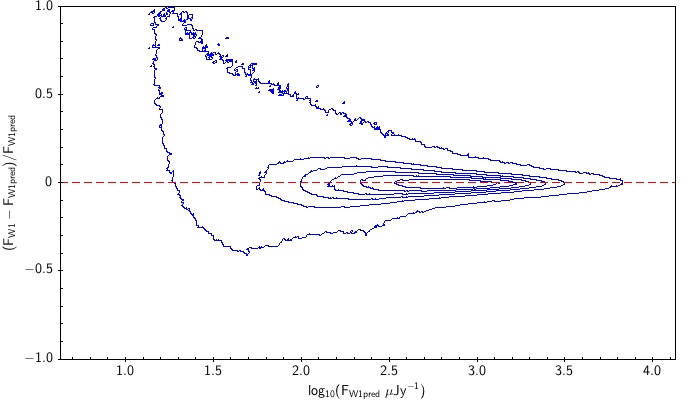
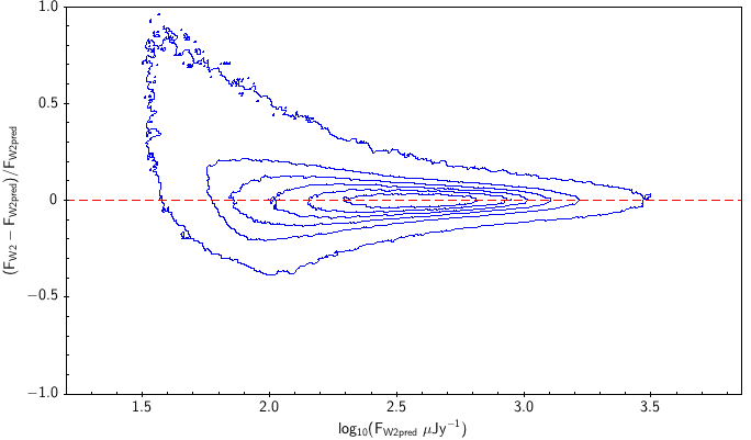
There is the remaining question of how well the models match the measured WISE fluxes. Figure 10 shows the source density distribution in fractional residual versus predicted flux space. In the case of ideal agreement, the red dashed line would hit the vertical tangent lines of the density curves. Missing on the high flux end is a disagreement in magnitude zero point (ie multiplicative offset). Missing on the low flux end is a background offset (i.e. additive offset). In more detail, the form is: $F_{\mathrm{corr}}={\mathrm{Zp}}_{\mathrm{corr}}\left(F_{\mathrm{obs}}+b\right).$ The values of ${\mathrm{Zp}}_{\mathrm{corr}}$ and $b$ that qualitatively align the distributions are in Table 6. Note how AllWISE requires less of a background offset than All–Sky.

Band	Subset	Uncorrected (a)	Corrected (b)
W1	AllWISE (1)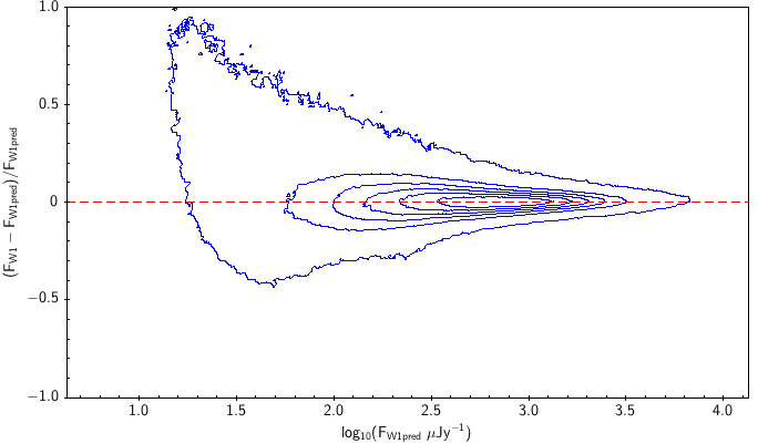
	WISE All–Sky (2)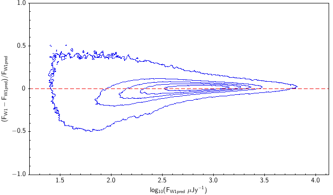
W2	AllWISE (3)
	WISE All–Sky (4)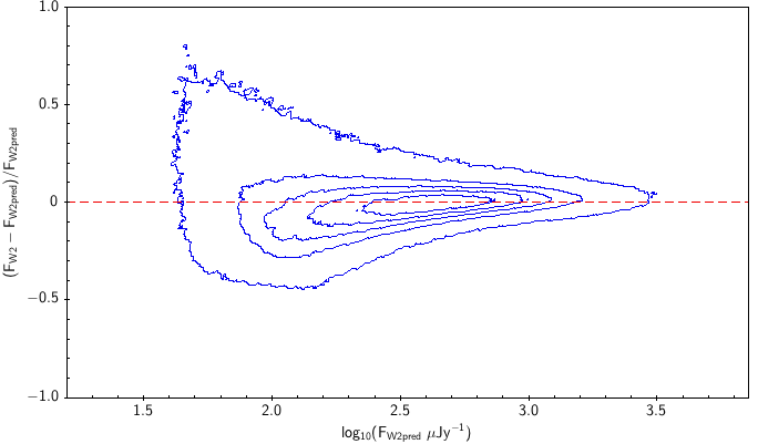
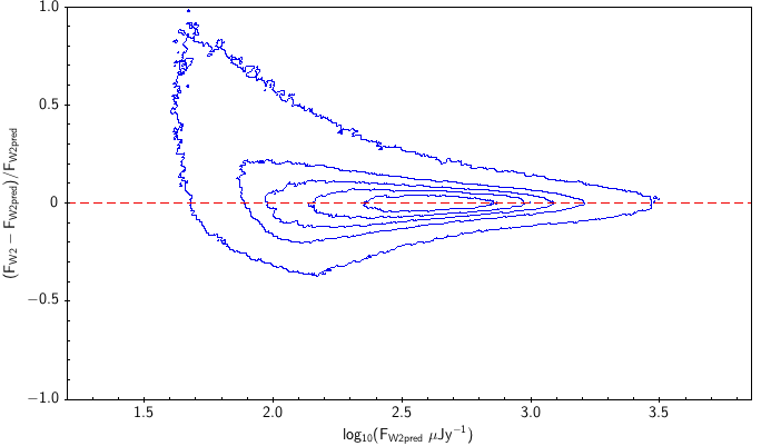Figure 10 – Fractional flux residual with level curves set by the density of points. The left column contains raw residuals, and the right column contains corrected residuals. The corrections are listed in Table 6. Note that the upward trend on the very faint end is a manifestation of Eddington bias.

Last update: 22 November 2013