VI. Analysis of Data Products
6. Catalog Reliability
d. Supplemental Reliability Figures
The process of evaluating the reliability of the All-Sky Release Source
Catalog produced a vast number of figures, most of which are unneeded for
arguing that the core reliability requirements are met, as discussed above.
However, they do provide additional insight into the catalog properties, so
a subset is presented here for additional background.
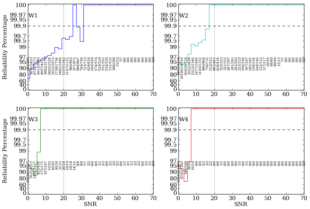
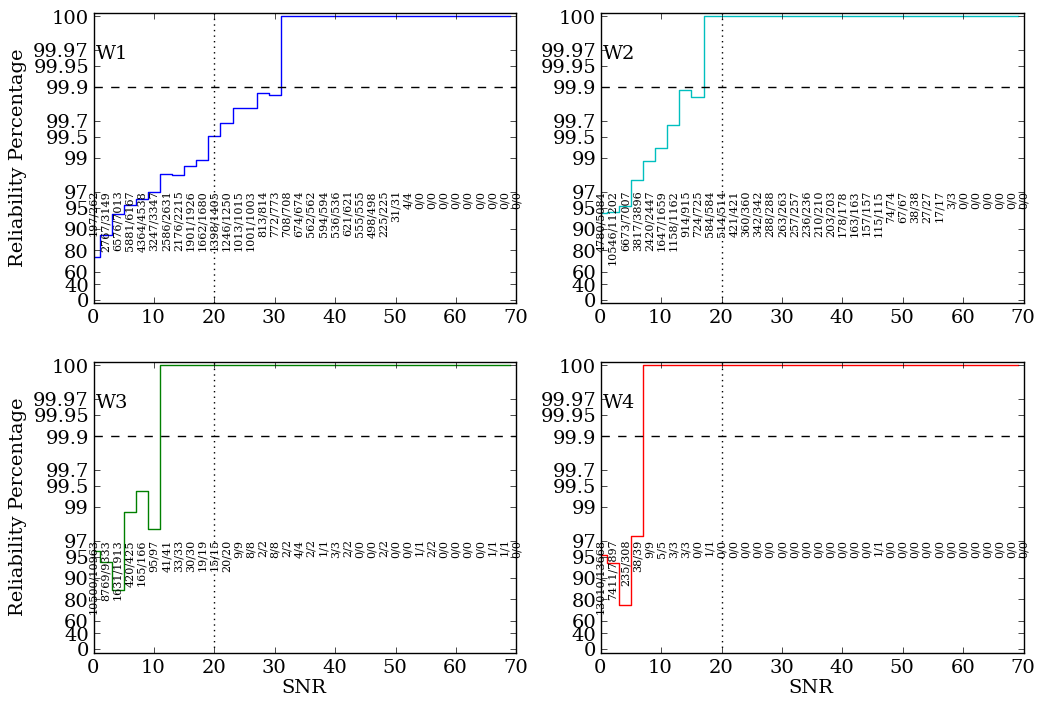
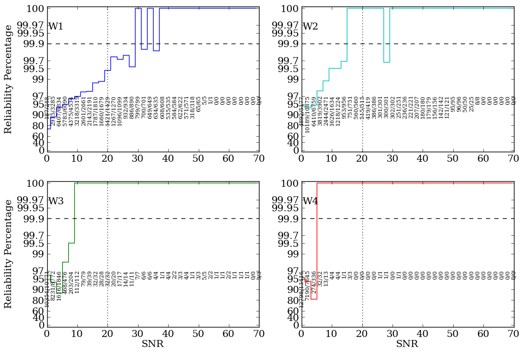
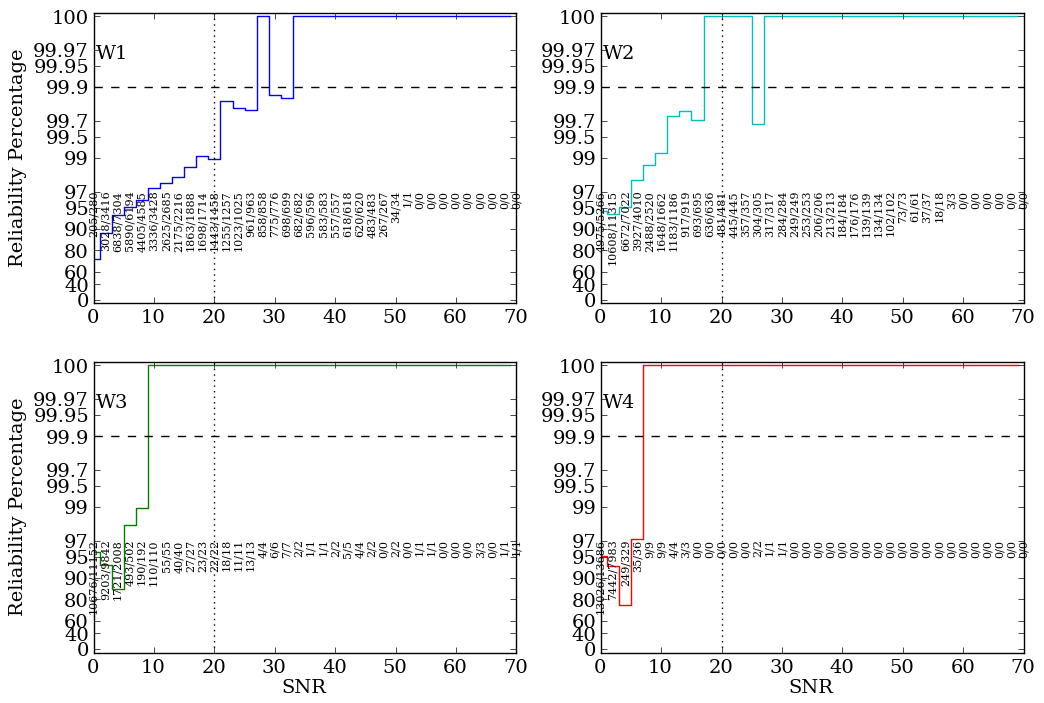
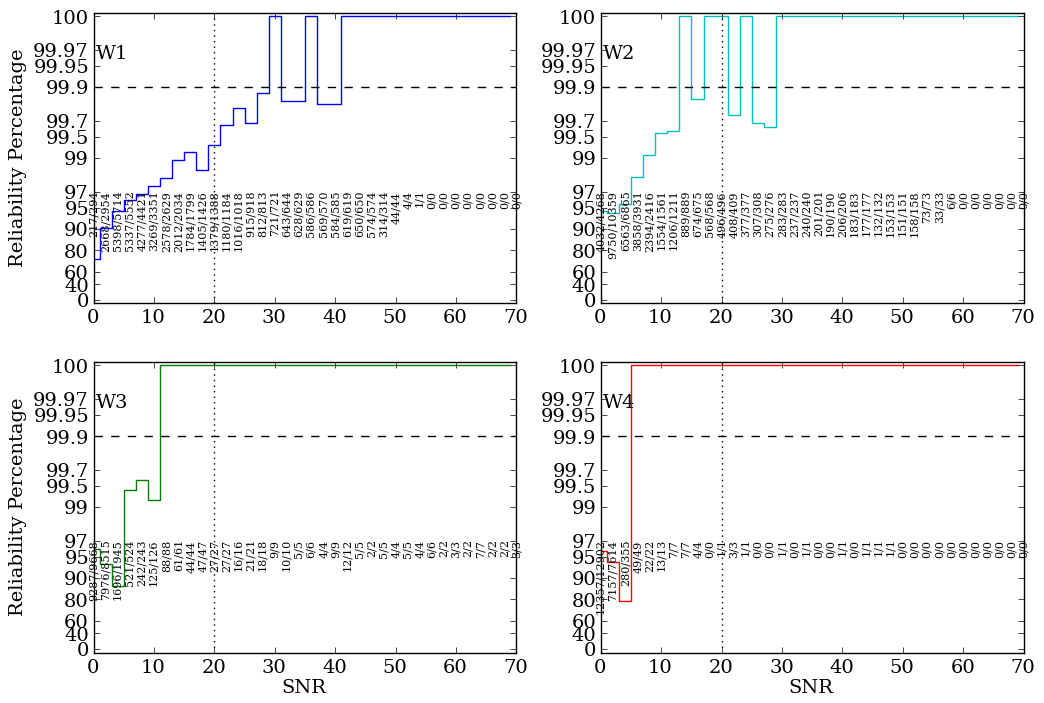
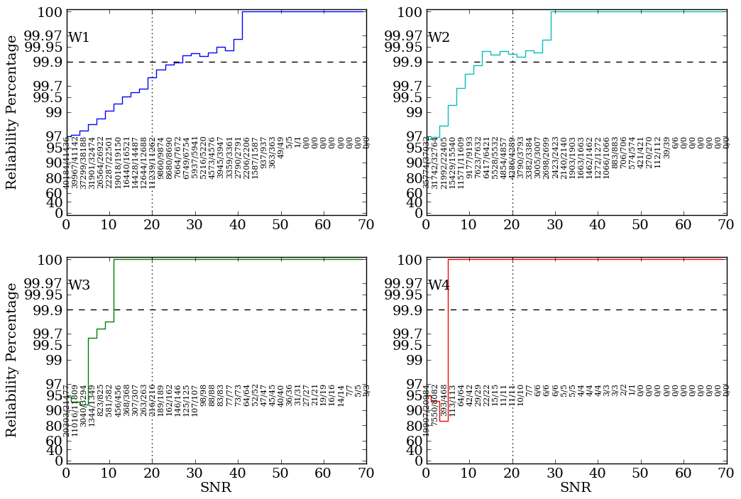
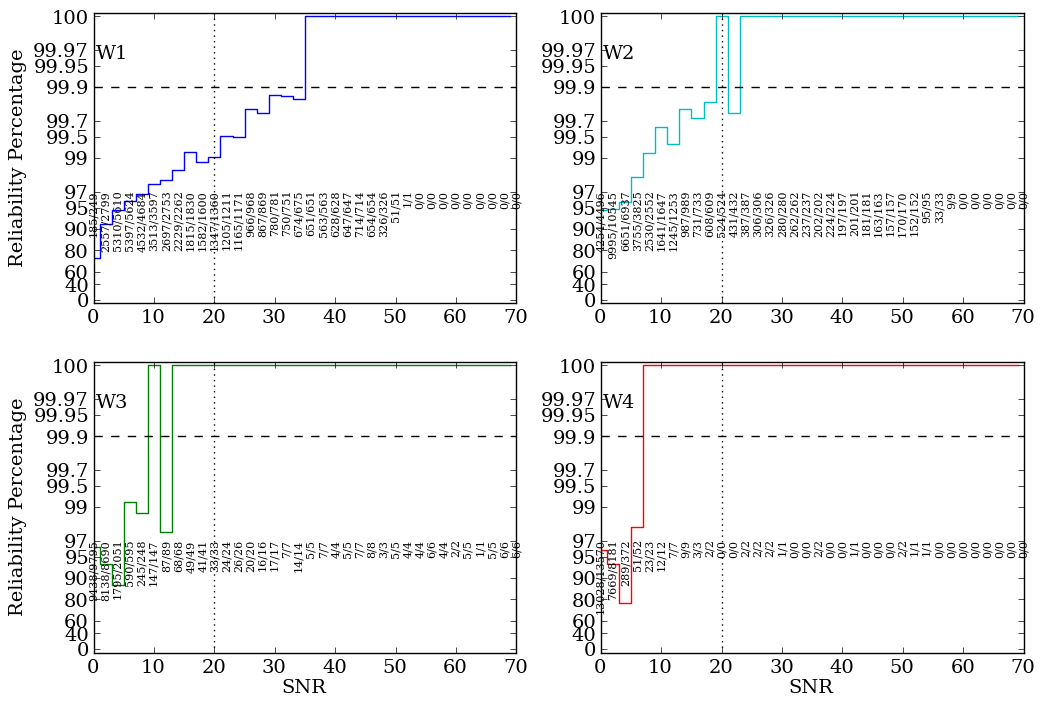
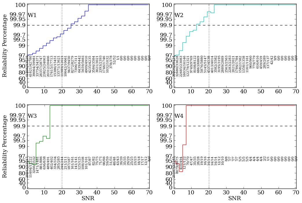
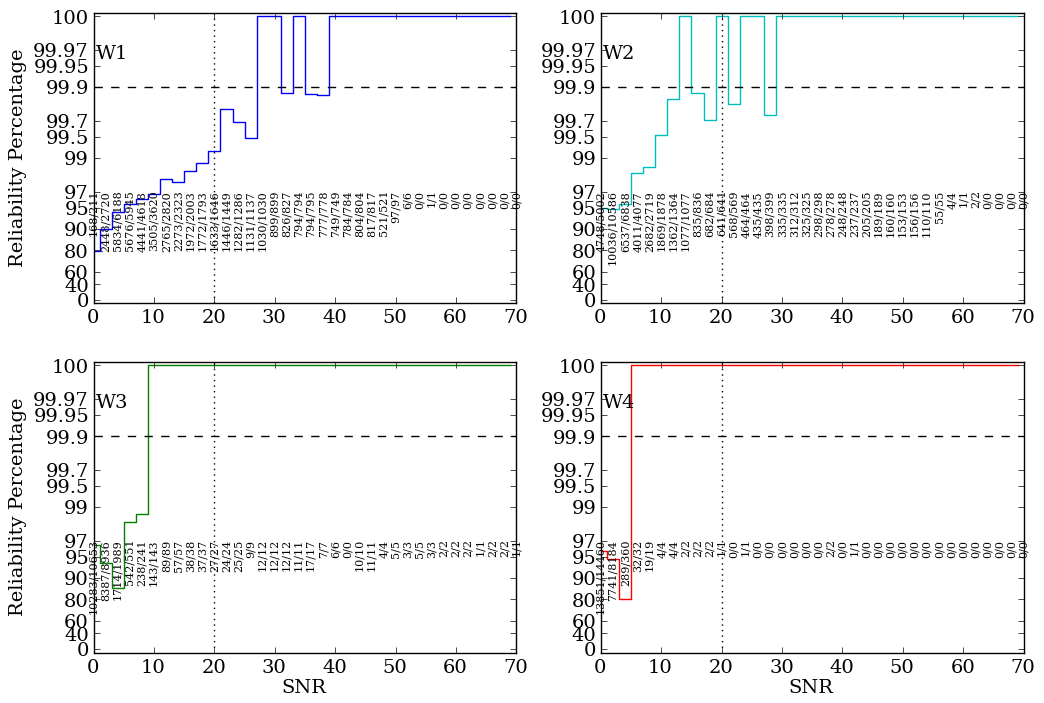
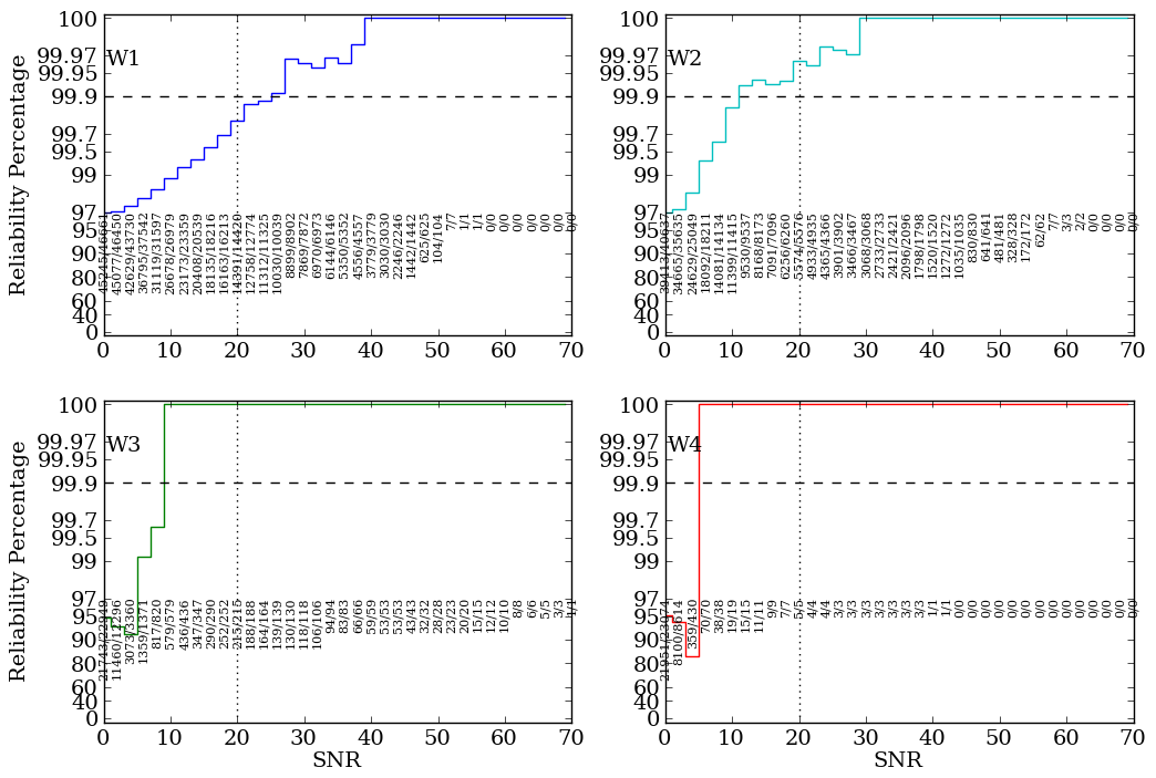
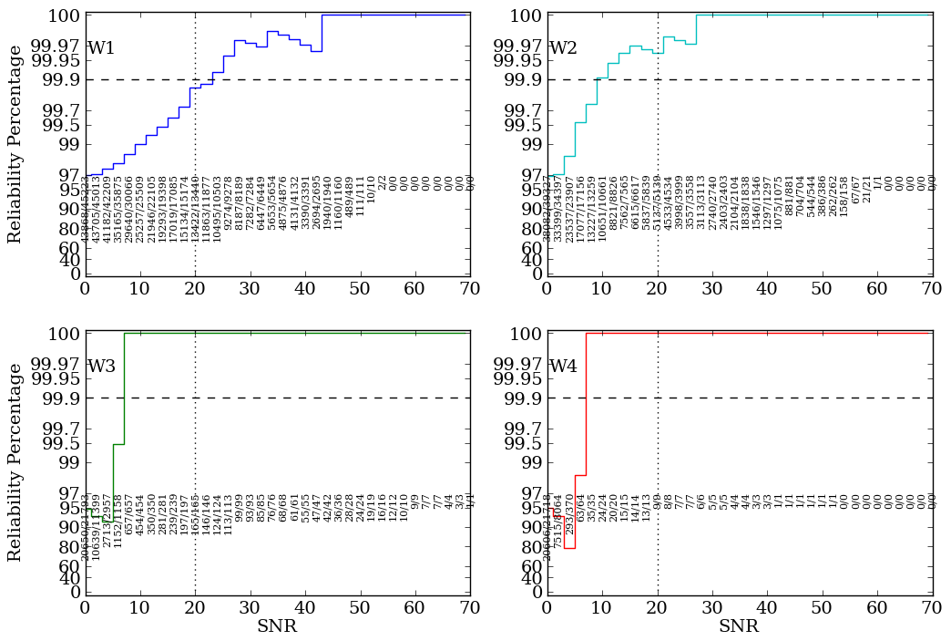
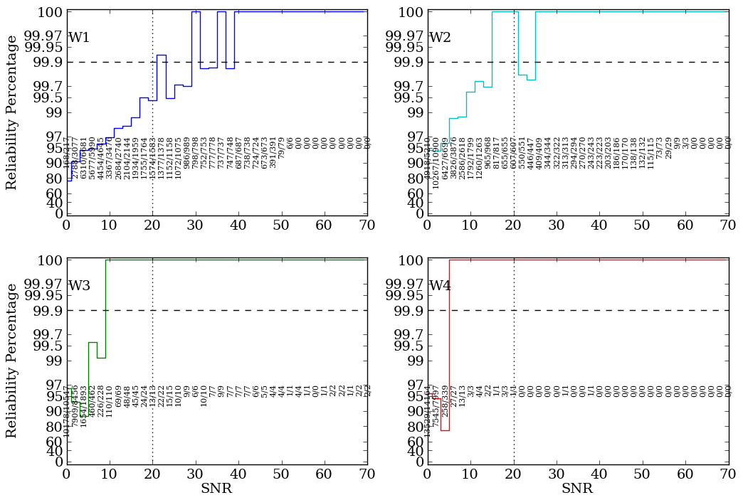
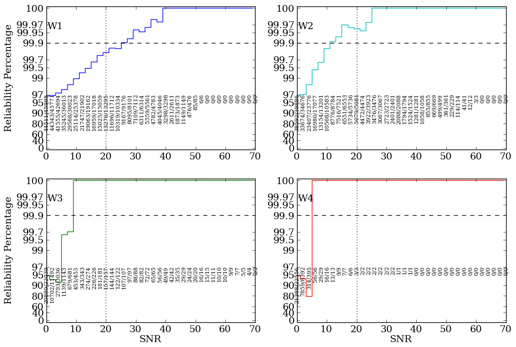
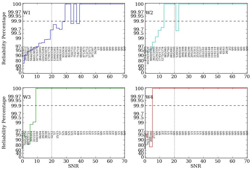
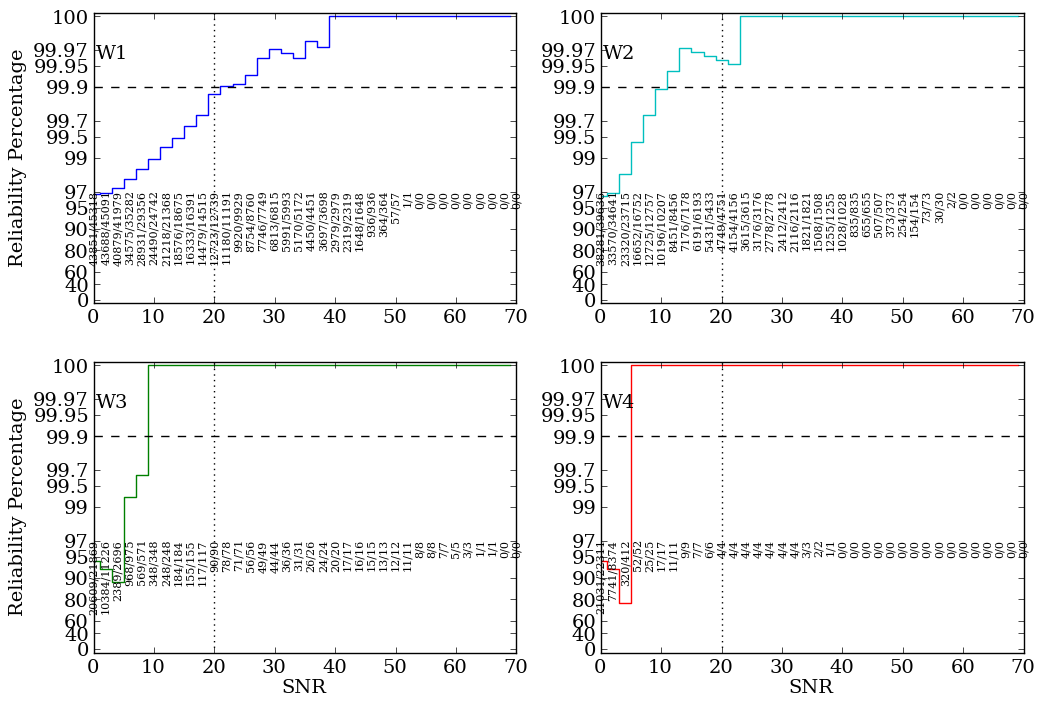
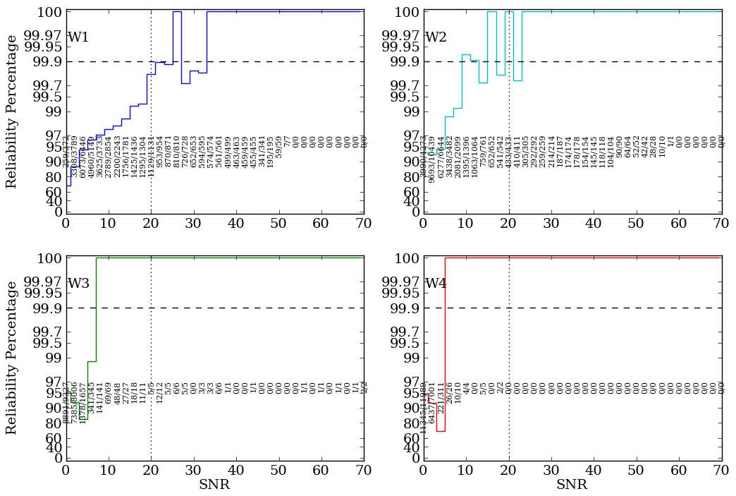
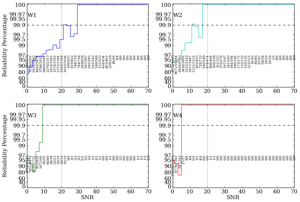
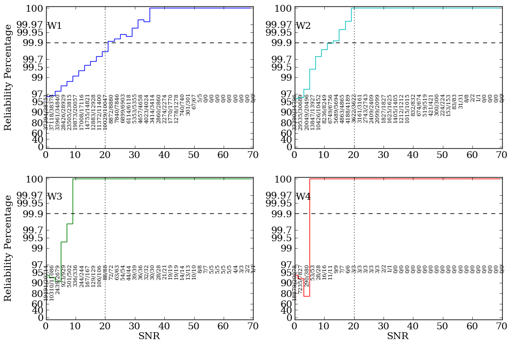
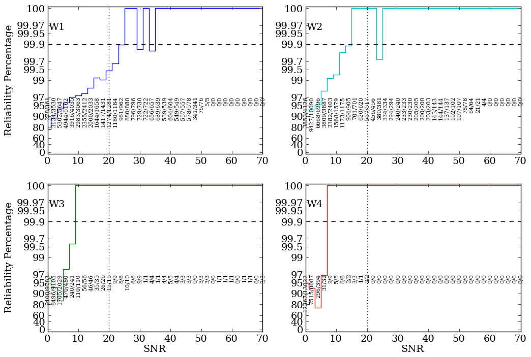
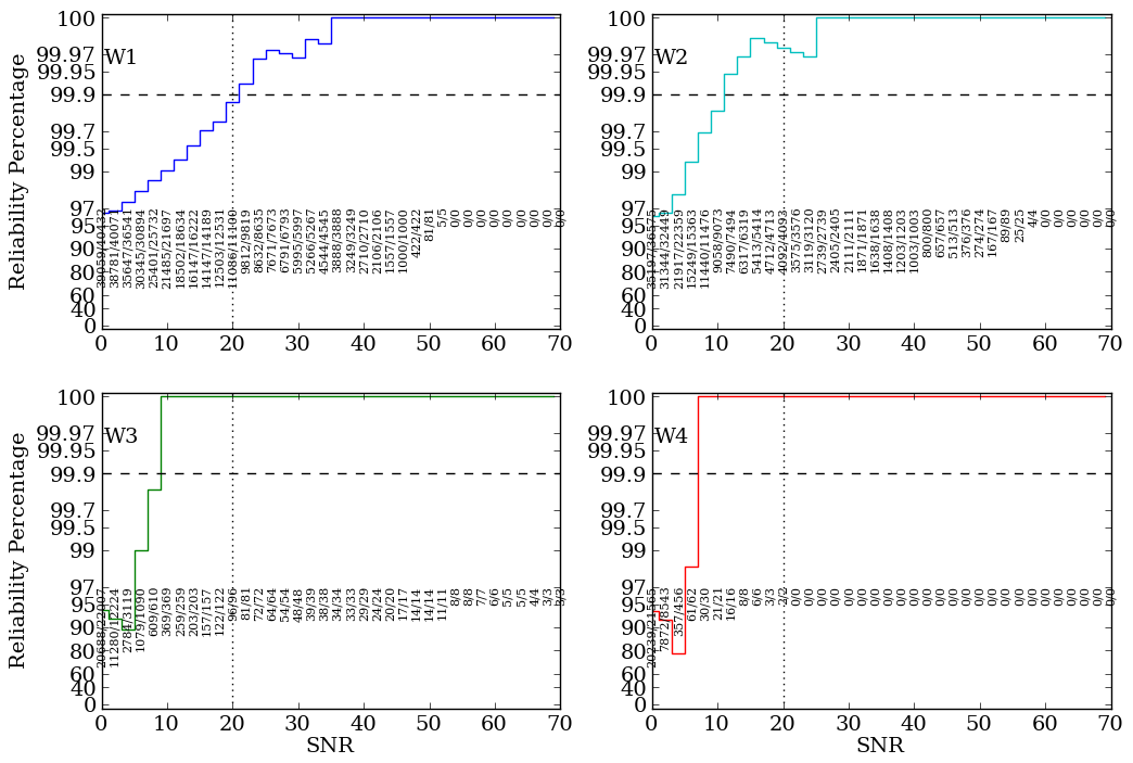
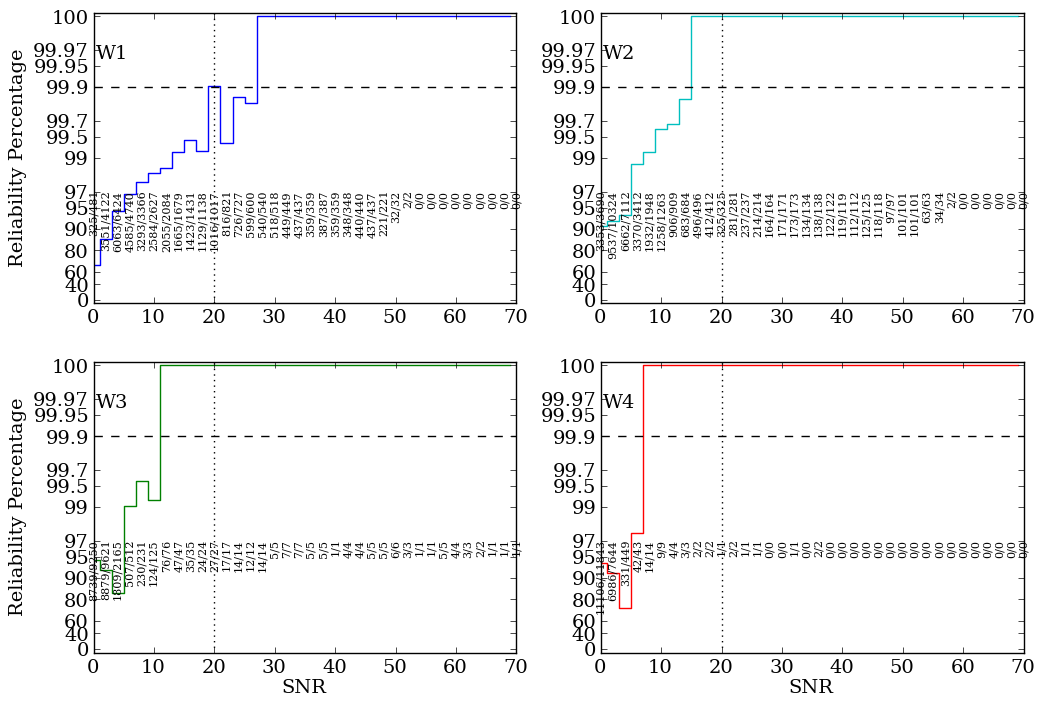
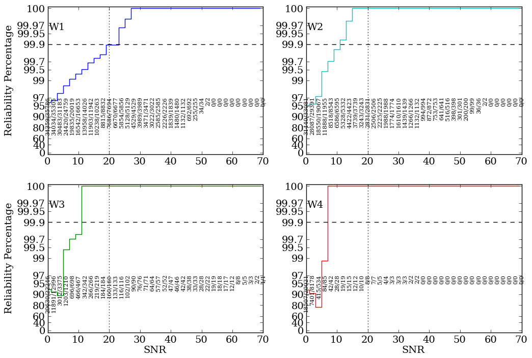
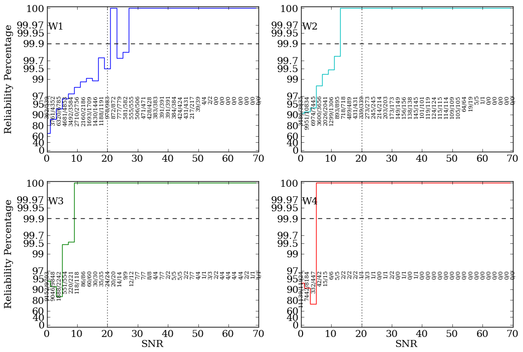
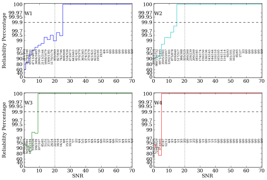
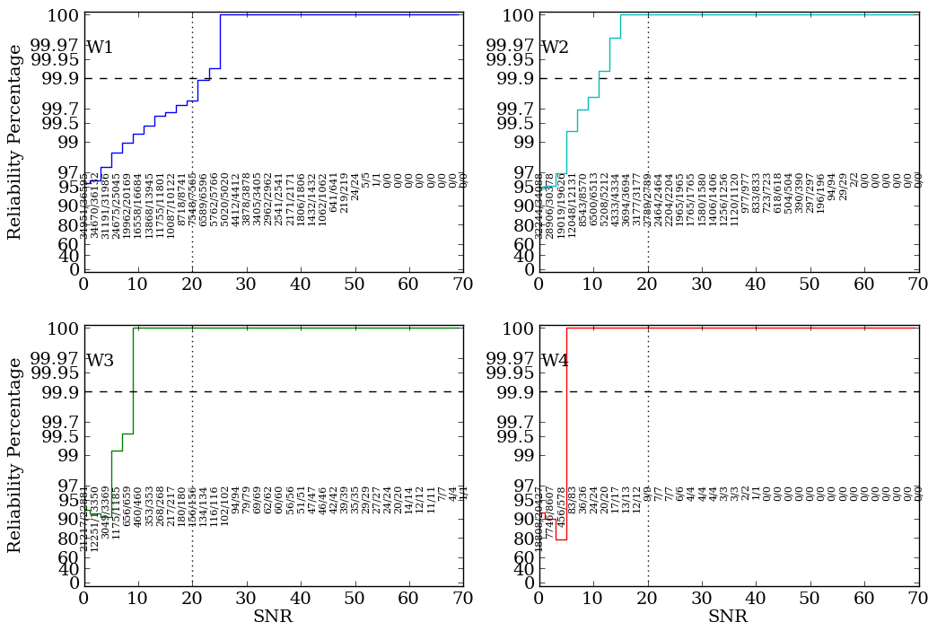
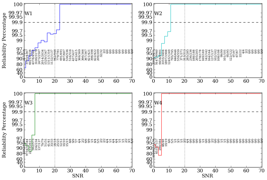
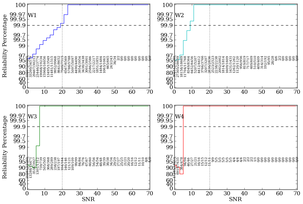
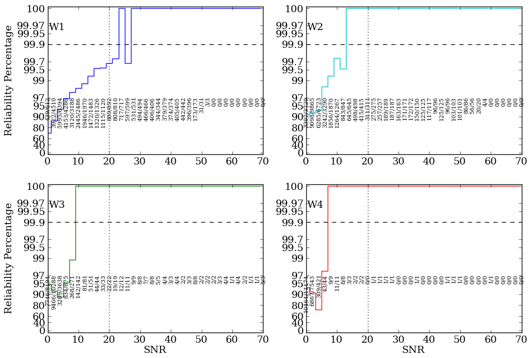
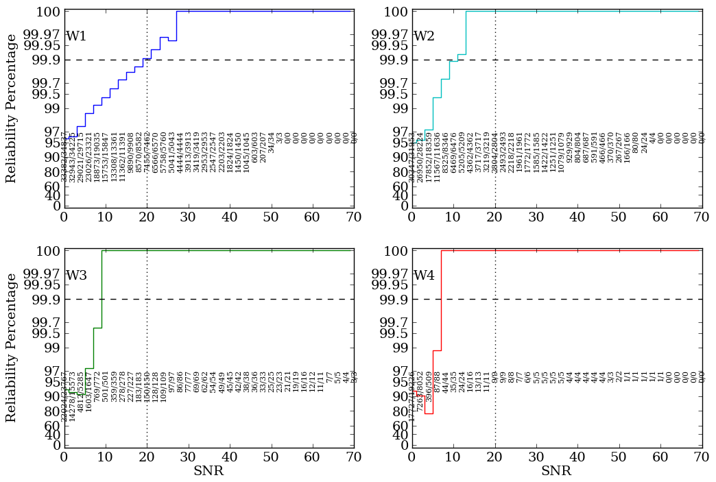
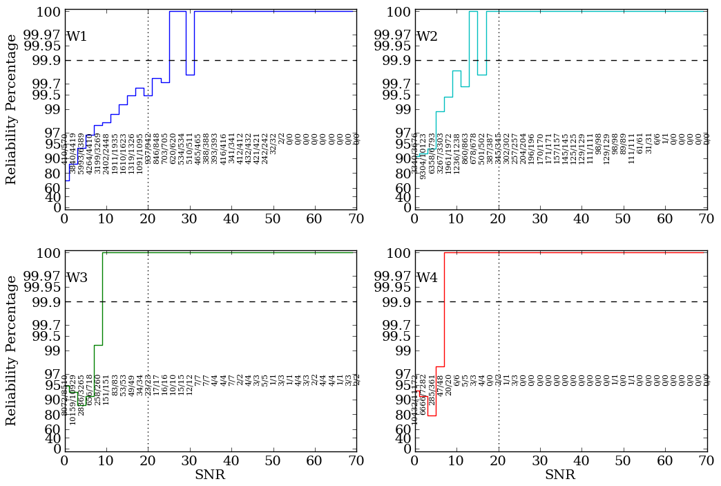
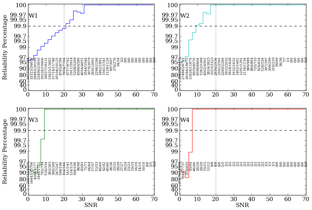
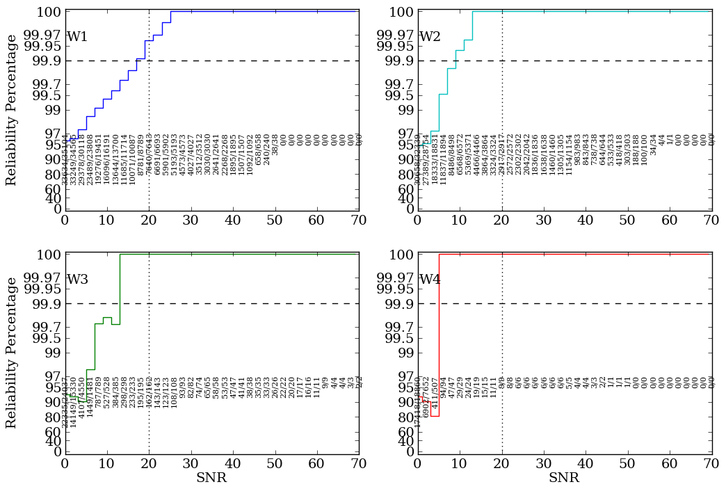
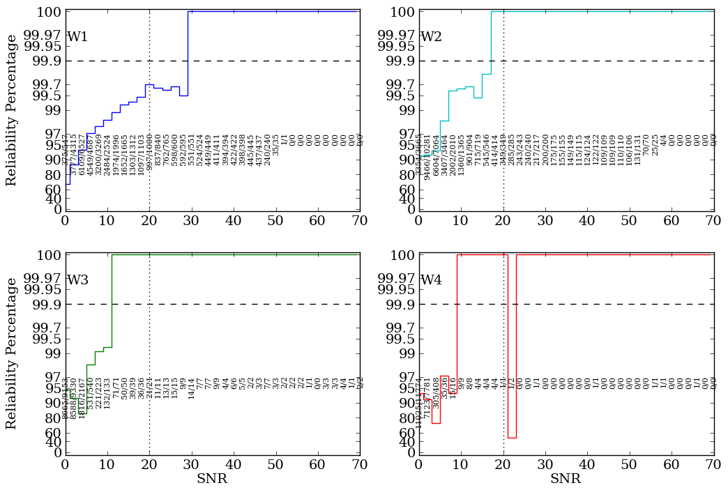
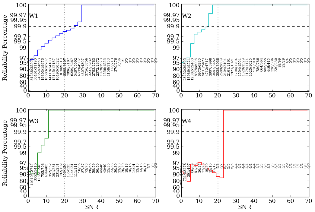
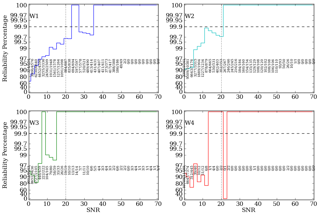
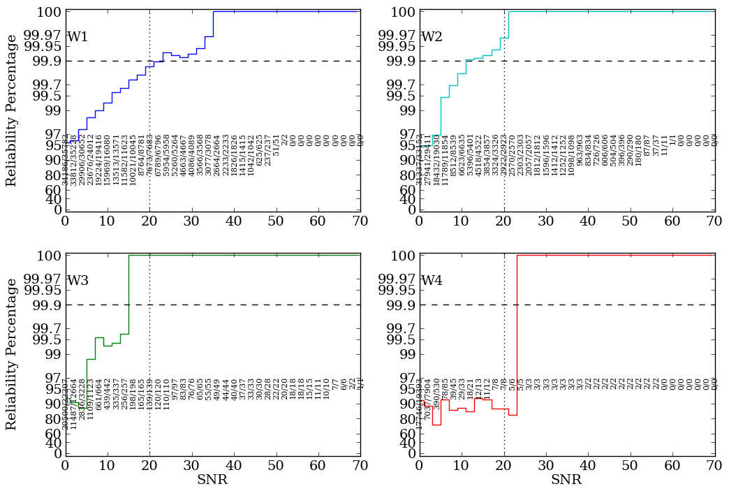
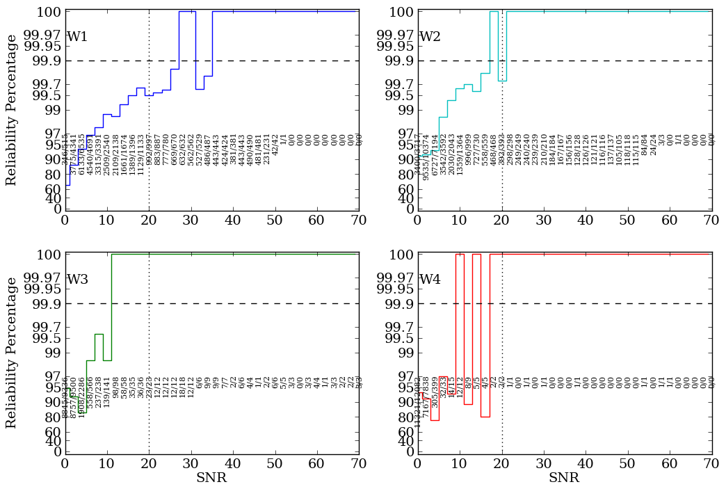
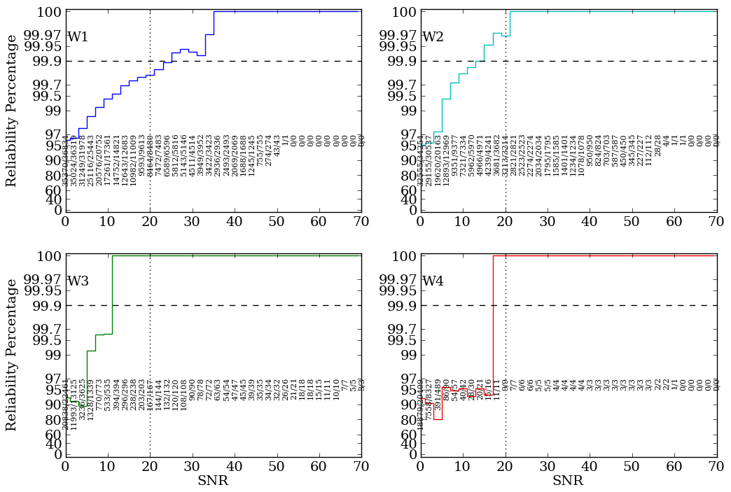
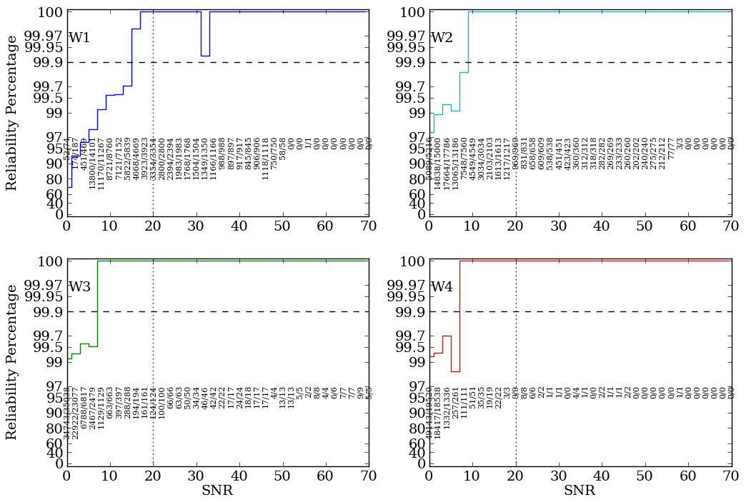
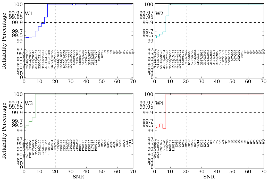
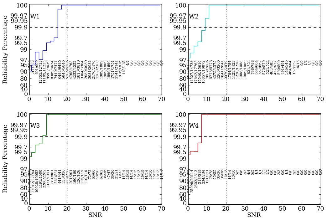
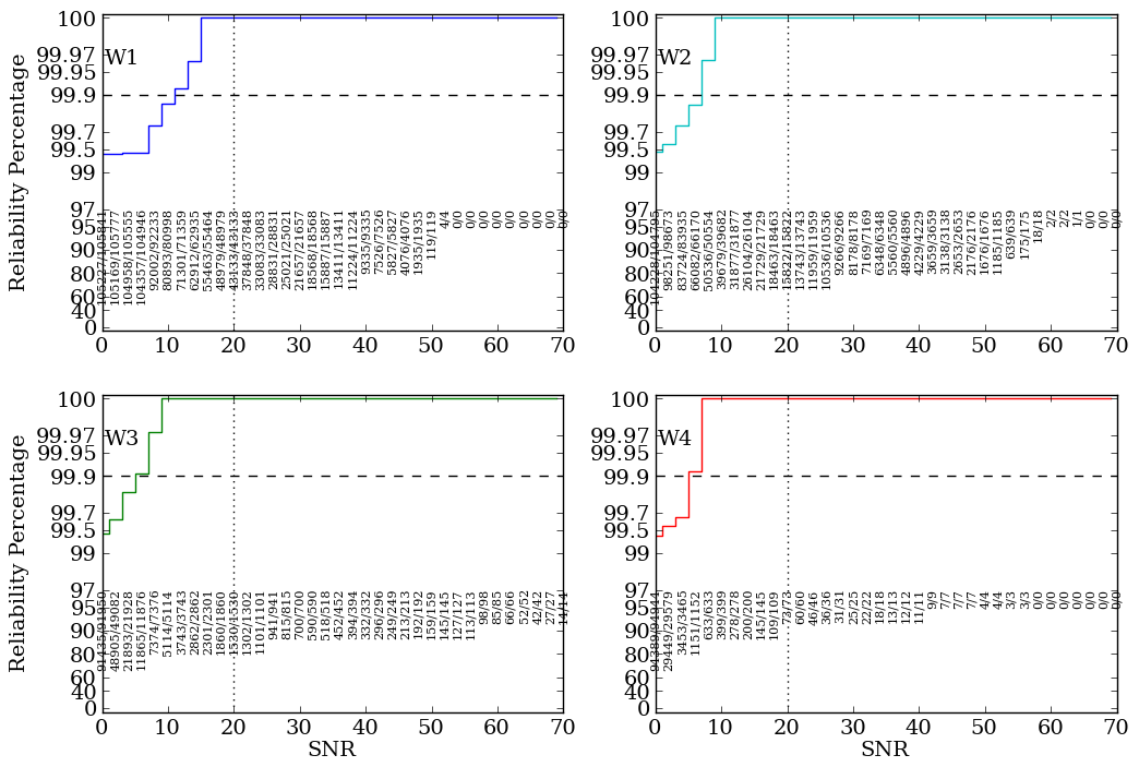
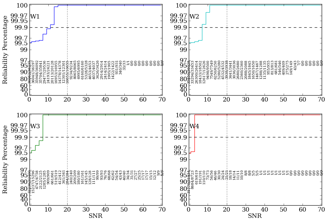
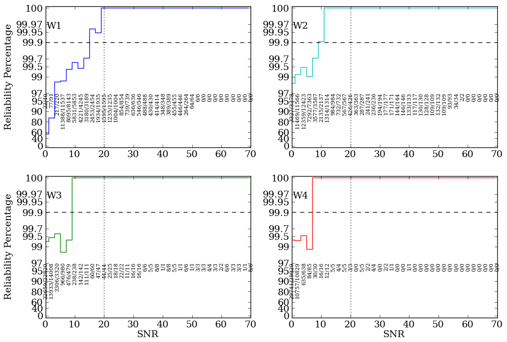
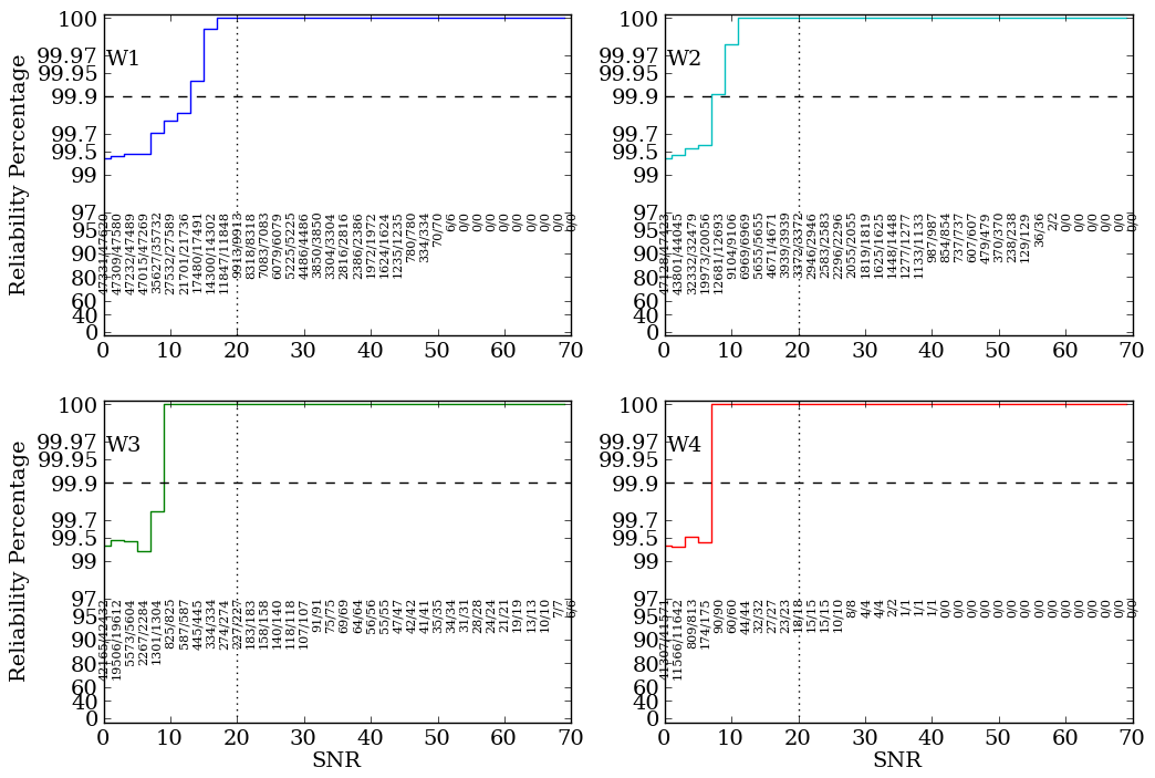
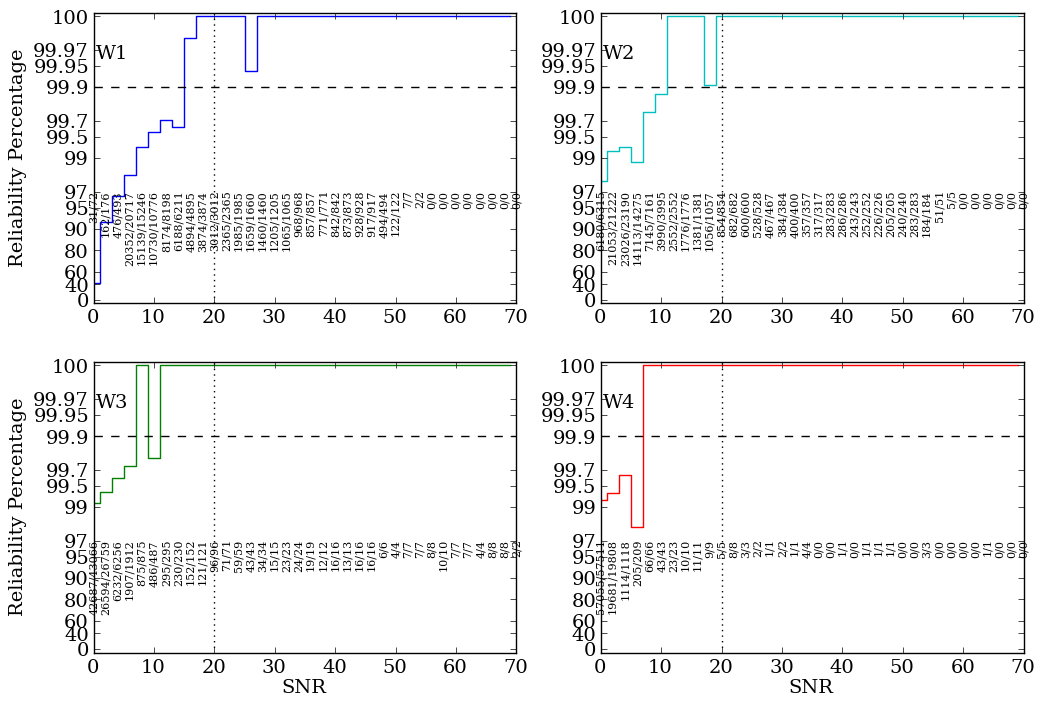
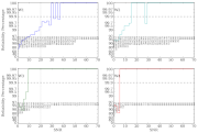
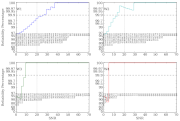
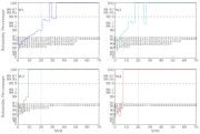
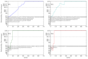
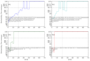
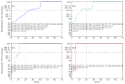
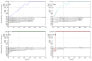
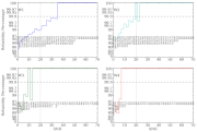
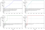
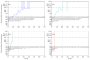
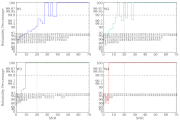
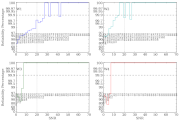
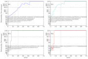
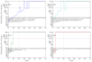
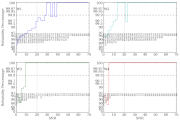
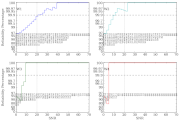
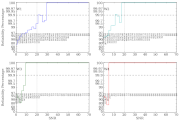
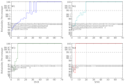
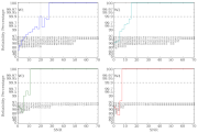
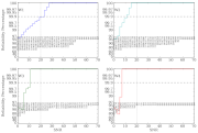
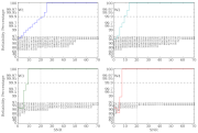
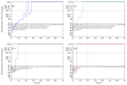
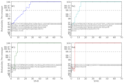
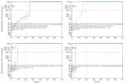
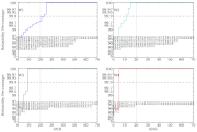
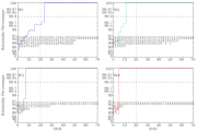
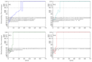
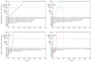
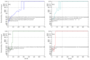
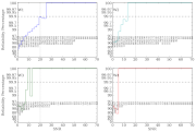
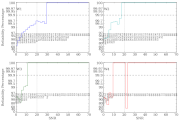
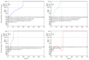
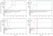
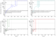
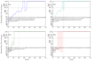
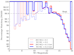
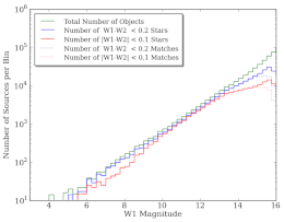
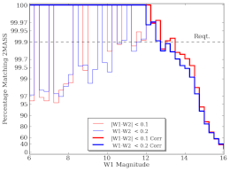
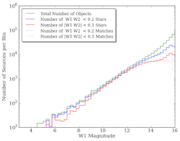
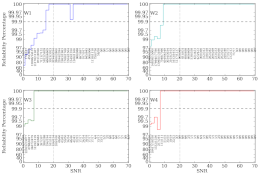
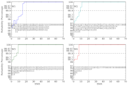
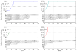
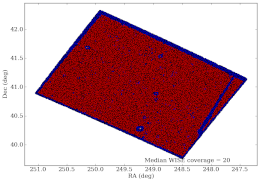
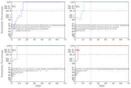
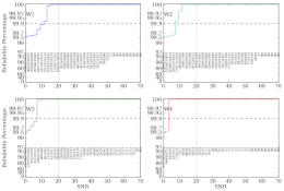
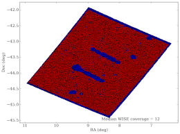
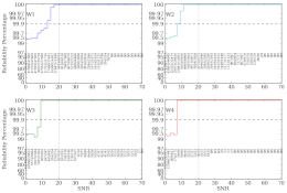
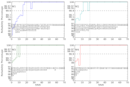
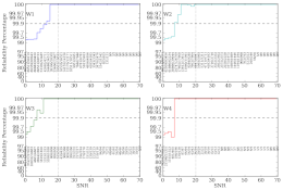
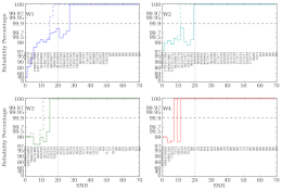
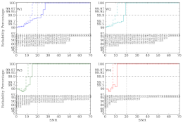
Internal Reliability Plots for Selected Variations of Each of the Seven Test Tiles
As mentioned in the main text, each of
the seven, 150-coverage, test tiles had ten, 15-coverage, coadds assembled
from the data. The reliability was measured for each of these 70 coadds and
the results were found to be quite consistent, especially after the blended
sources were filtered out. To present evidence of that consistency, four
variations of each of the seven test tiles are presented here. Variations 0,
3, 5, and 8 were chosen at random.
Except for a single W4 source in two of the 2741p636 tile variations
(which turns out to be part of the resolved planetary nebula DS Dra [K
1-16]; so it should, in fact, be classified as a reliable detection), 99.9%
reliability is demonstrated for all the variations for W2, W3, and W4 for
SNR ≥ 20. In W1, 99.9% is occasionally exceeded, but most typically it
falls at 99.8% for SNR ≥ 20. It never lies below 99.7%. We take this as
evidence that the truth table itself (the deep WISE coadd) is limited to
99.9% reliability at W1.
| Differential | Cumulative | Differential | Cumulative |
 |
 |
 |
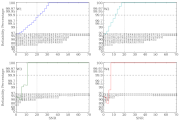 |
| 0825m637_nm10_00 |
0825m637_nm10_03 |
 |
 |
 |
 |
| 0825m637_nm10_05 |
0825m637_nm10_08 |
| Figures 1a-1h (left to right) |
| Differential | Cumulative | Differential | Cumulative |
 |
 |
 |
 |
| 0891m637_nm10_00 |
0891m637_nm10_03 |
 |
 |
 |
 |
| 0891m637_nm10_05 |
0891m637_nm10_08 |
| Figures 2a-2h (left to right) |
| Differential | Cumulative | Differential | Cumulative |
 |
 |
 |
 |
| 0949m682_nm10_00 |
0949m682_nm10_03 |
 |
 |
 |
 |
| 0949m682_nm10_05 |
0949m682_nm10_08 |
| Figures 3a-3h (left to right) |
| Differential | Cumulative | Differential | Cumulative |
 |
 |
 |
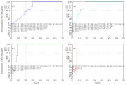 |
| 0988m682_nm10_00 |
0988m682_nm10_03 |
 |
 |
 |
 |
| 0988m682_nm10_05 |
0988m682_nm10_08 |
| Figures 4a-4h (left to right) |
| Differential | Cumulative | Differential | Cumulative |
 |
 |
 |
 |
| 2675p636_nm10_00 |
2675p636_nm10_03 |
 |
 |
 |
 |
| 2675p636_nm10_05 |
2675p636_nm10_08 |
| Figures 5a-5h (left to right) |
| Differential | Cumulative | Differential | Cumulative |
 |
 |
 |
 |
| 2708p636_nm10_00 |
2708p636_nm10_03 |
 |
 |
 |
 |
| 2708p636_nm10_05 |
2708p636_nm10_08 |
| Figures 6a-6h (left to right) |
| Differential | Cumulative | Differential | Cumulative |
 |
 |
 |
 |
| 2741p636_nm10_00 |
2741p636_nm10_03 |
 |
 |
 |
 |
| 2741p636_nm10_05 |
2741p636_nm10_08 |
| Figures 7a-7h (left to right) |
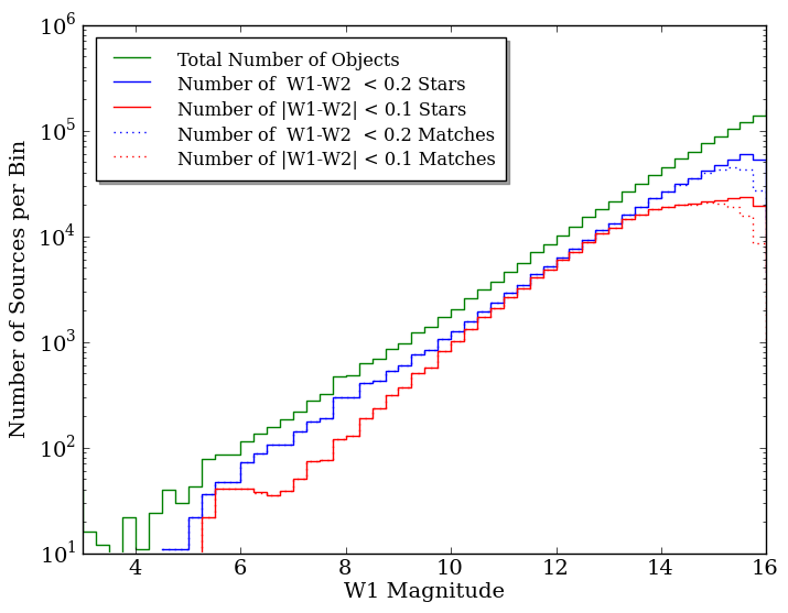
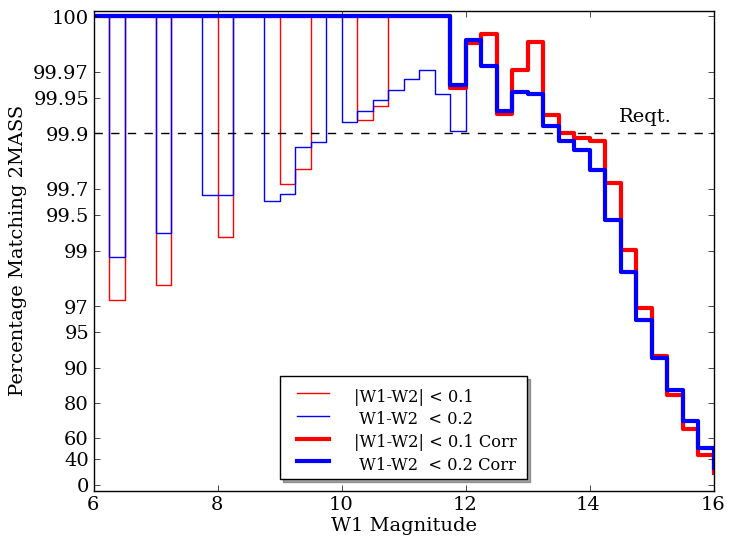
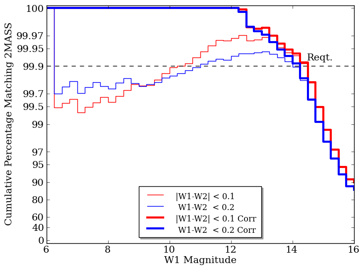
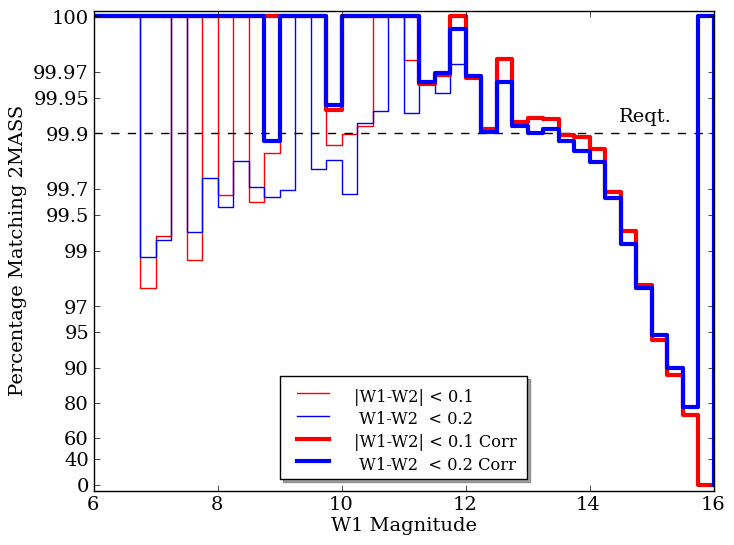
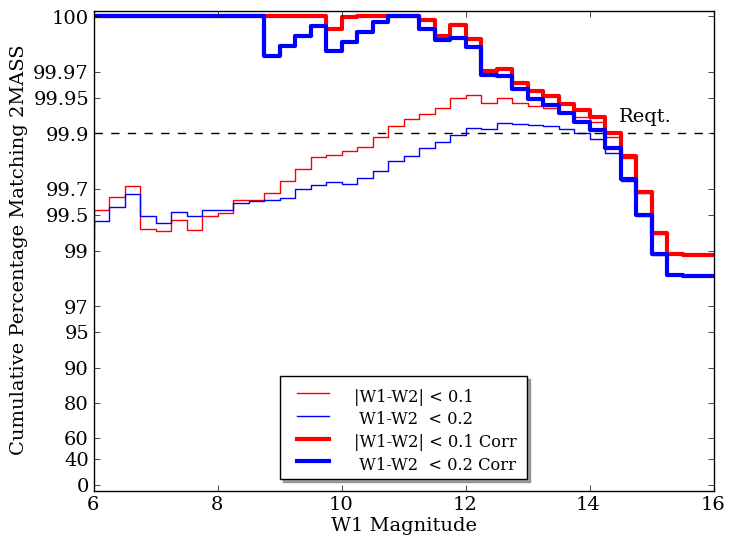
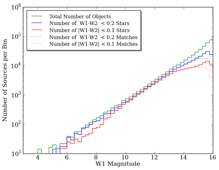
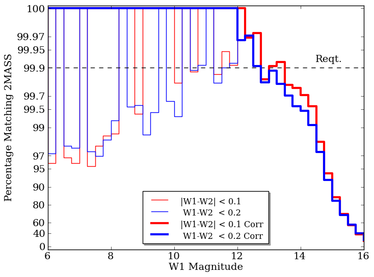
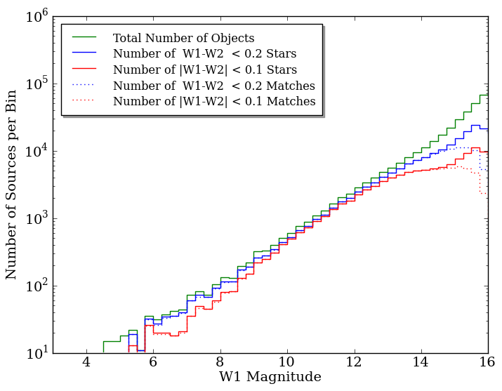
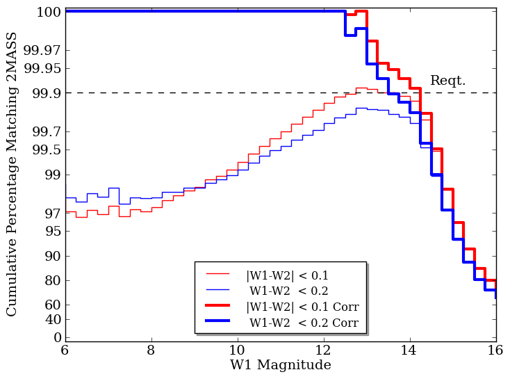
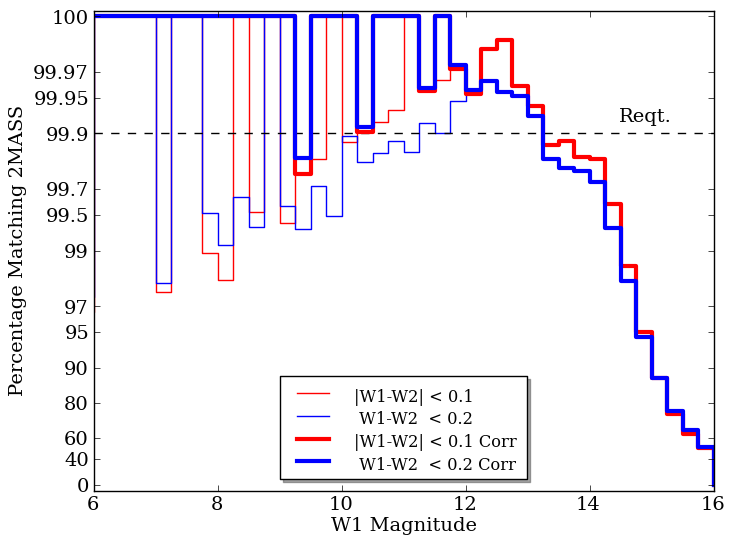
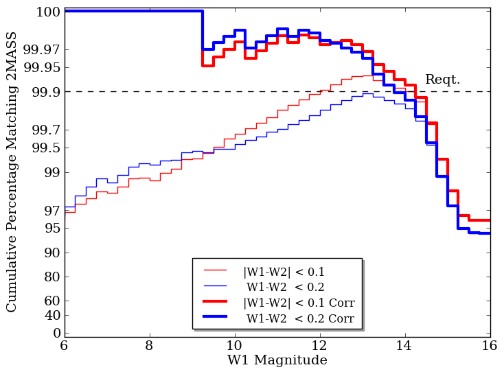
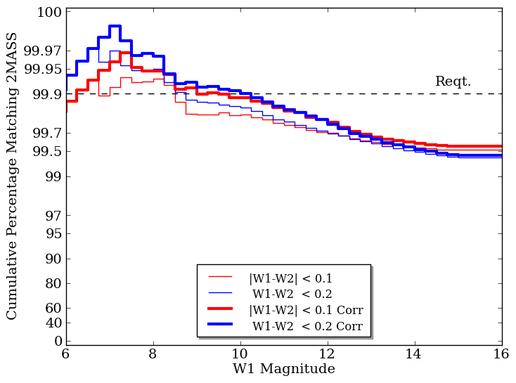
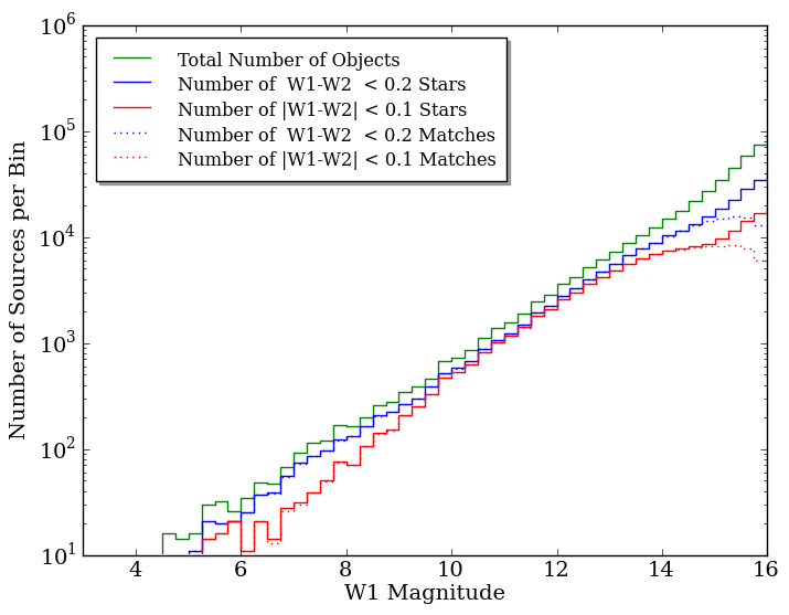
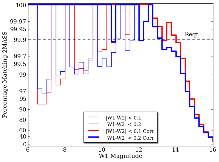
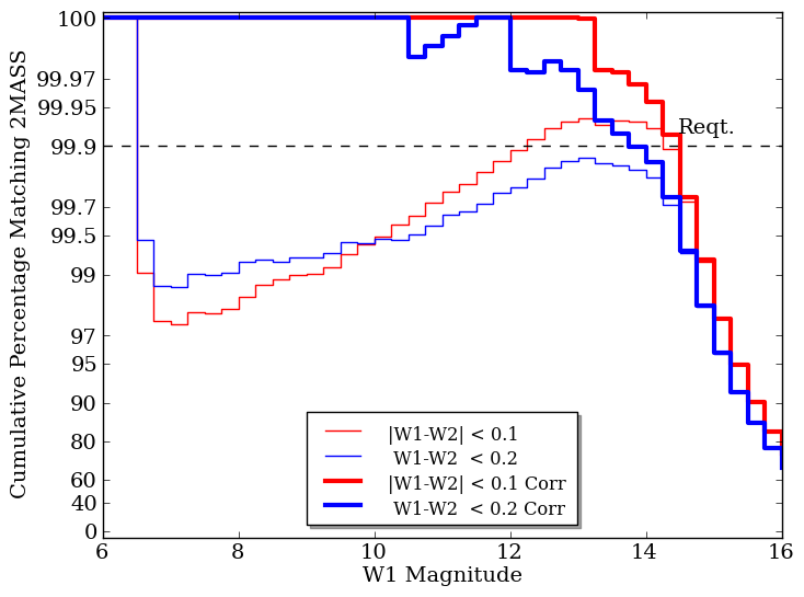
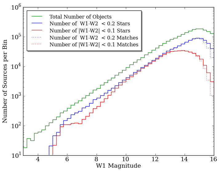
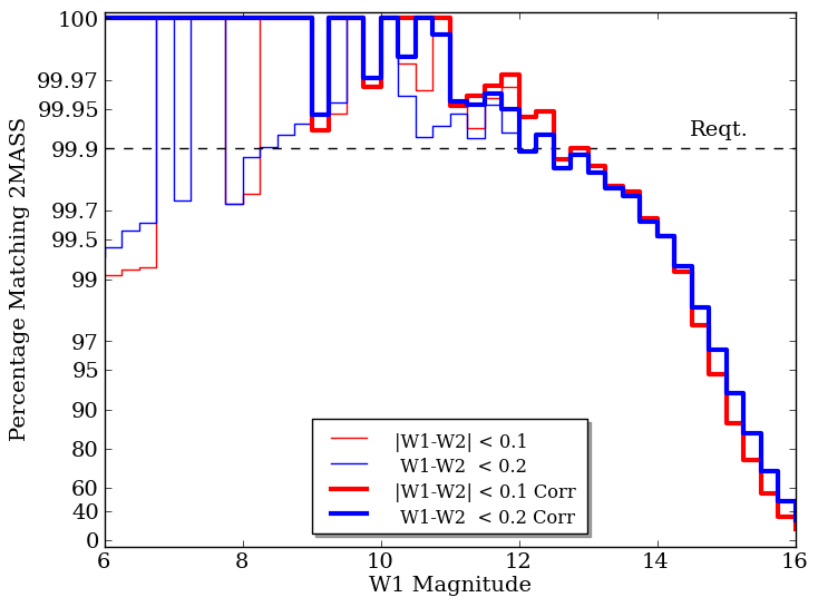
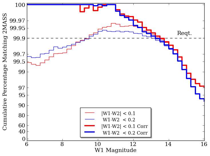
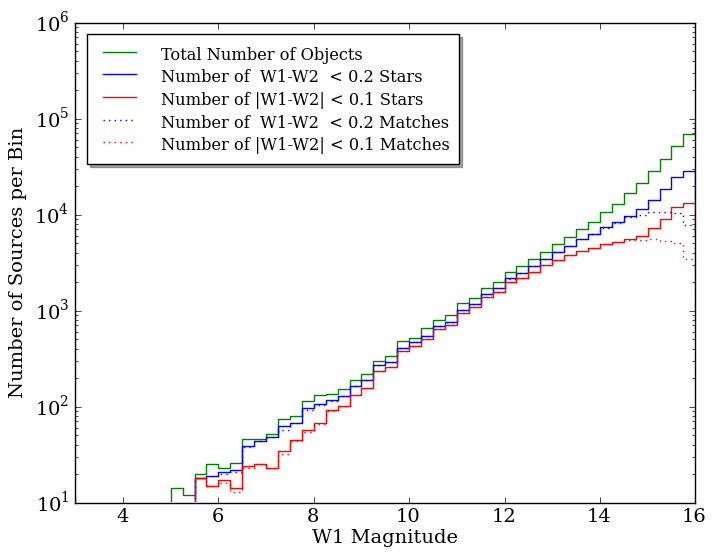
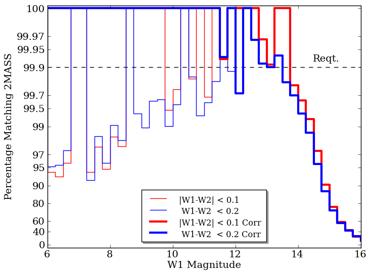
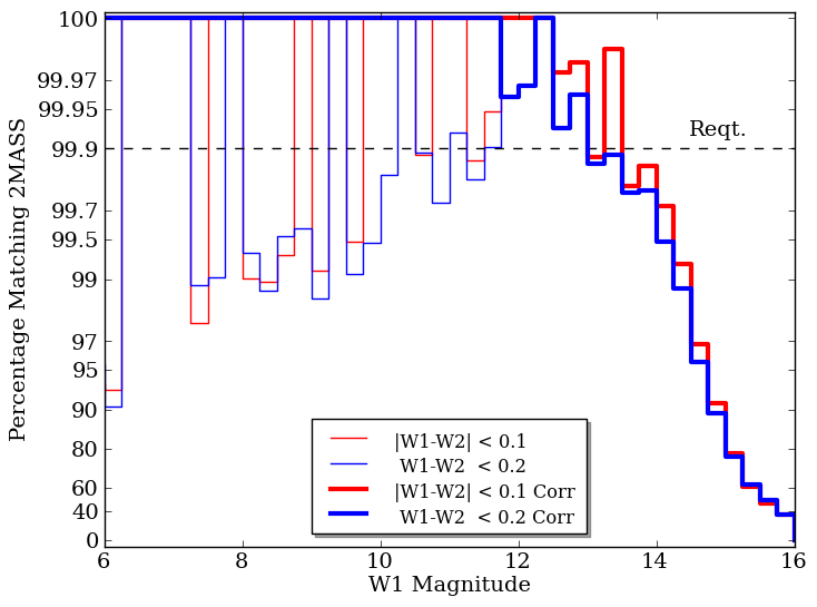
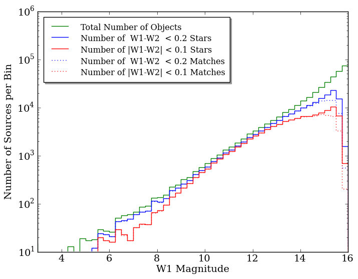
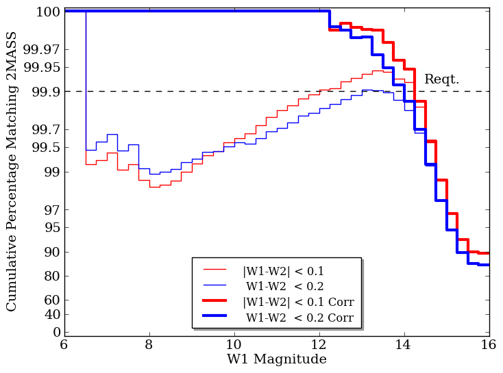
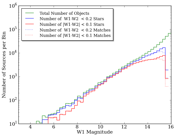
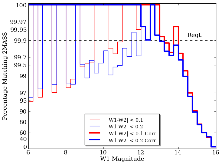
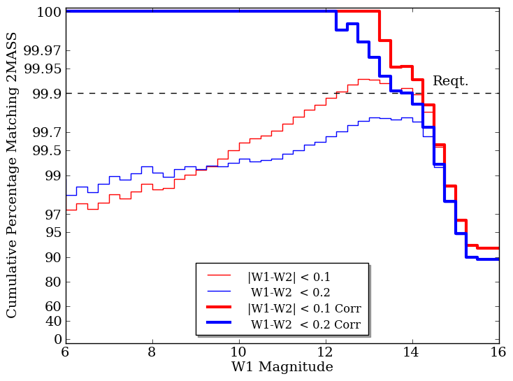
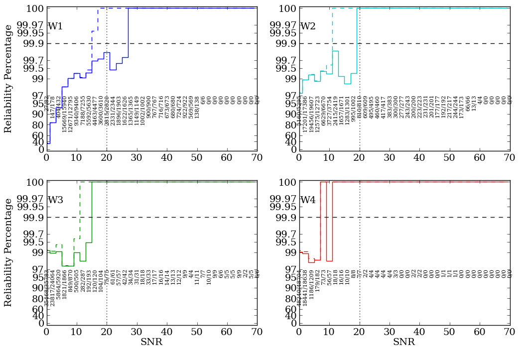
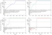
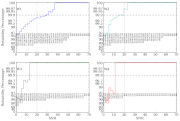
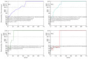
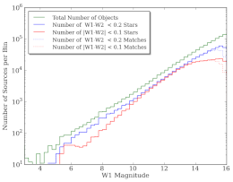
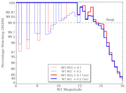
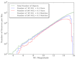
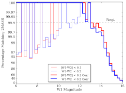
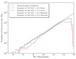
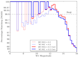
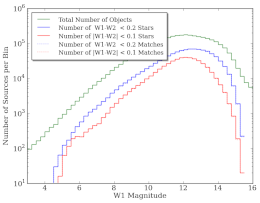
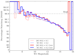
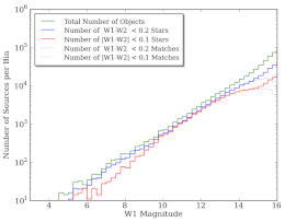
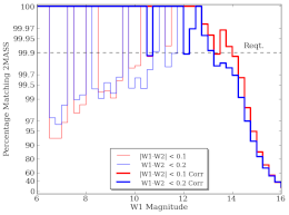
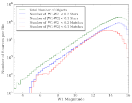
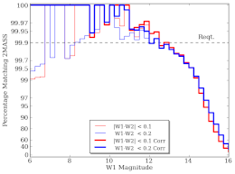
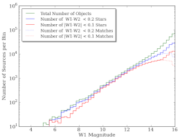
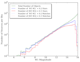
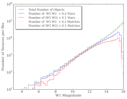
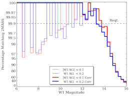
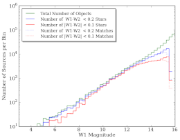
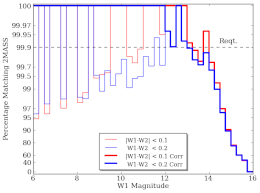
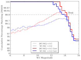
2MASS Reliability Plots for Individual WISE Test Regions
The plots shown in the main WISE/2MASS comparison are the sum of all the
sources found in 11 of the 12 test regions. Because each region has a
somewhat different environment, all 12 regions are plotted here
individually. All show good behavior for sources as faint as W1 = 14 except
for Region 6. The processing and plotting format is identical to
the main WISE/2MASS comparison section.
 |
 |
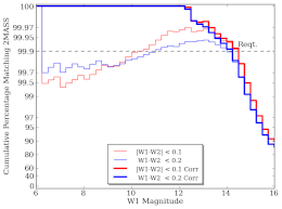 |
Figure 8a - Test Region 1 number counts.
(South equatorial pole) |
Figure 8b - Differential reliability. |
Figure 8c - Cumulative reliability. |
 |
 |
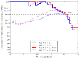 |
Figure 9a - Test Region 2 number counts.
(Ecliptic plane, complex field – Taurus) |
Figure 9b - Differential reliability. |
Figure 9c - Cumulative reliability. |
 |
 |
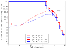 |
Figure 10a - Test Region 3 number counts.
(High galactic latitude – SDSS Overlap) |
Figure 10b - Differential reliability. |
Figure 10c - Cumulative reliability. |
 |
 |
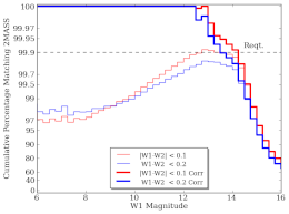 |
Figure 11a - Test Region 4 number counts.
(High galactic latitude – CDF-s) |
Figure 11b - Differential reliability. |
Figure 11c - Cumulative reliability. |
 |
 |
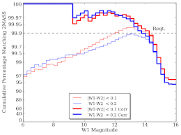 |
Figure 12a - Test Region 5 number counts.
(Low ecliptic latitude, M67) |
Figure 12b - Differential reliability. |
Figure 12c - Cumulative reliability. |
 |
 |
 |
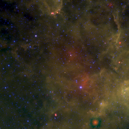
Figure 13a - Test Region 6 number counts.
(Galactic plane) |
Figure 13b - Differential reliability. |
Figure 13c - Cumulative reliability. |
 |
 |
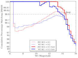 |
Figure 14a - Test Region 7 number counts.
(ELAIS-N1) |
Figure 14b - Differential reliability. |
Figure 14c - Cumulative reliability. |
 |
 |
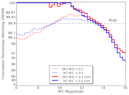 |
Figure 15a - Test Region 8 number counts.
(Low galactic latitude – Cepheus) |
Figure 15b - Differential reliability. |
Figure 15c - Cumulative reliability. |
 |
 |
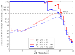 |
Figure 16a - Test Region 9 number counts.
(Bootes) |
Figure 16b - Differential reliability. |
Figure 16c - Cumulative reliability. |
 |
 |
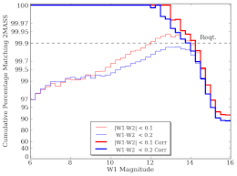 |
Figure 17a - Test Region 10 number counts.
(COSMOS) |
Figure 17b - Differential reliability. |
Figure 17c - Cumulative reliability. |
 |
 |
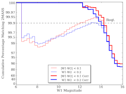 |
Figure 18a - Test Region 11 number counts.
(South Pole Telescope survey field) |
Figure 18b - Differential reliability. |
Figure 18c - Cumulative reliability. |
 |
 |
 |
| Figure 19a - Test Region 12 number counts. (Coordinate origin, Jupiter) |
Figure 19b - Differential reliability. |
Figure 19c - Cumulative reliability. |
Test Region 6 (Galactic Plane) was excluded from the 2MASS comparison
statistics due to the overwhelming number of sources contained within it and
the corresponding confusion. The number count plot begins to deviate from a
power law near 10th magnitude, at far brighter levels than in any other
field. Even Test Region 8 (b = +5°), though it has a significant amount
of nebulosity, has far fewer sources and a correspondingly fainter turn-off.
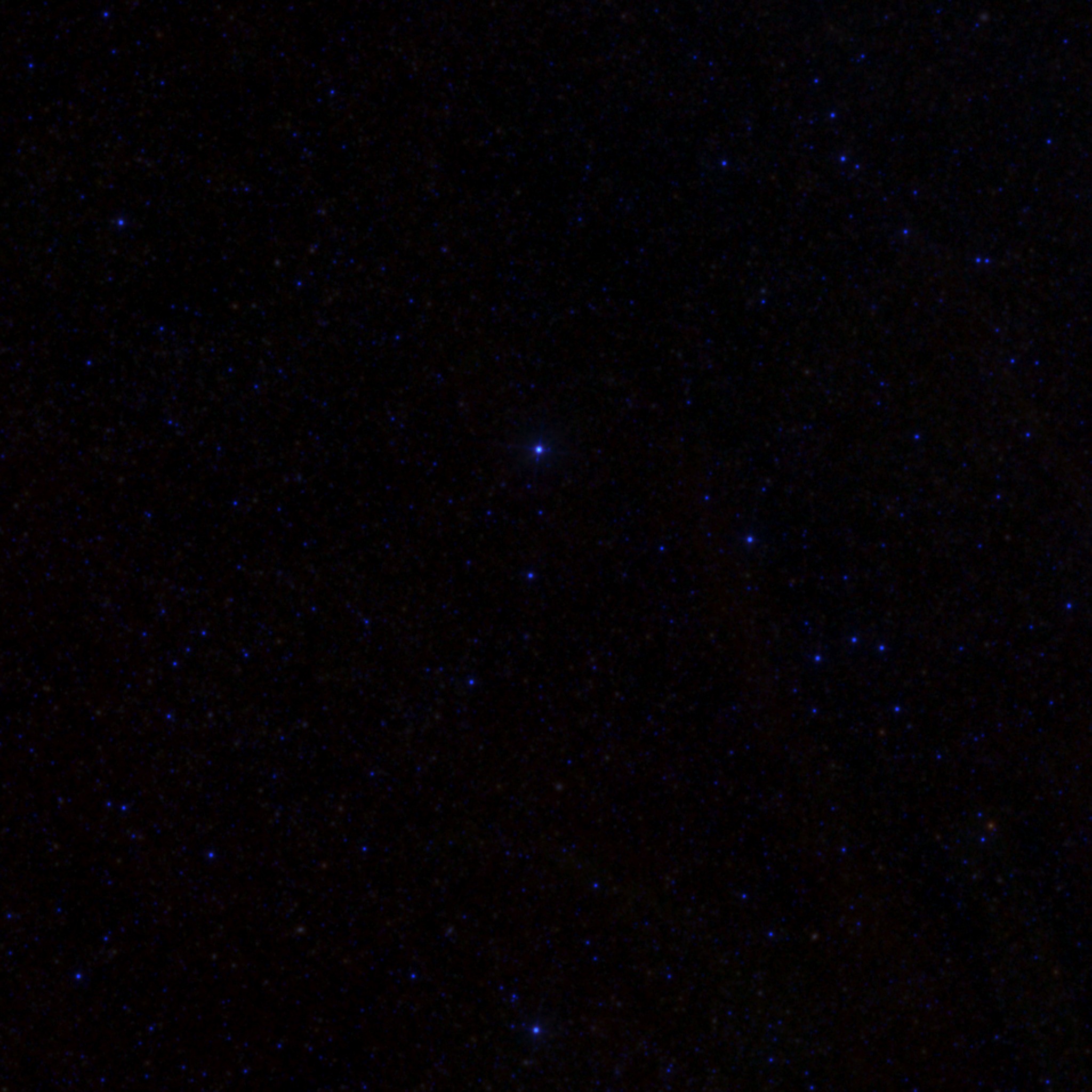
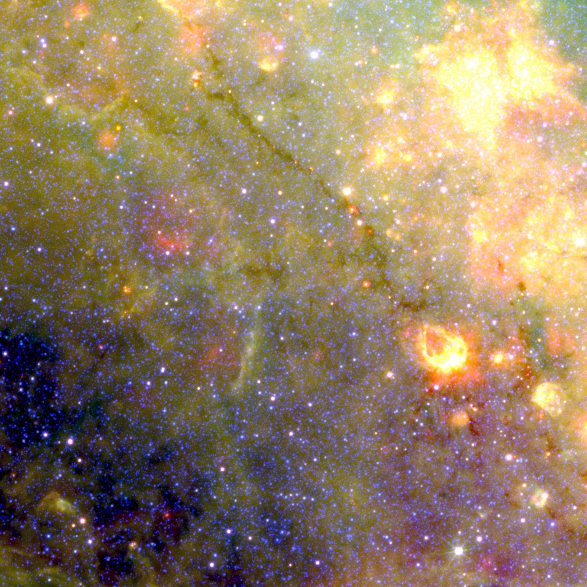
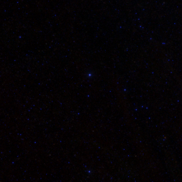
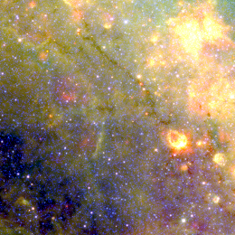
Below are the central tiles for Regions 7, 8, and 6, all processed and
scaled in an identical manner. The density of sources in Region 6 is so high
that the confusion in W1 makes it difficult to see (or extract)
sources fainter than 10th magnitude.
 |
 |
 |
| Figure 20a - Test Region 7 (ELAIS-N1). |
Figure 20b - Test Region 8 (Cepheus). |
Figure 20c - Test Region 6 (Galactic plane). |
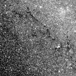 |
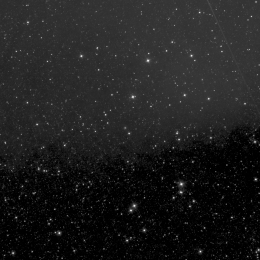
| Figure 21 - W1 image from Test Region 6. |
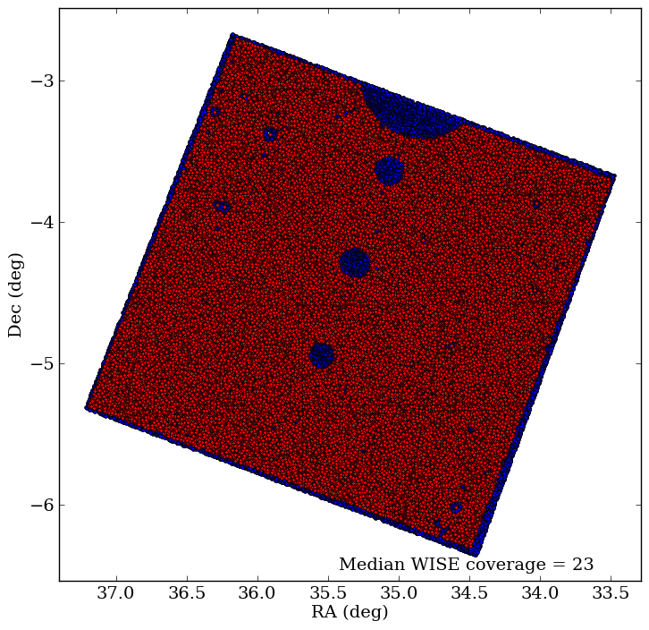
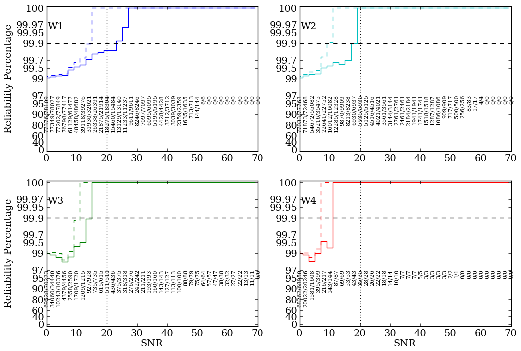
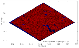
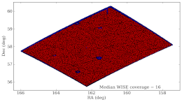
Additional Spitzer Comparison Regions
Data for the six Spitzer SWIRE fields are presented here. The results match
those of the COSMOS field with the exception of the XMM field, which will be
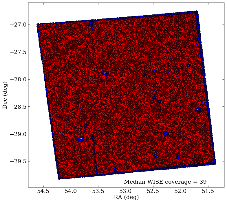
discussed after its plot. The "holes" and "slots" in the WISE coverage maps
are due to artifact flagging from bright star halos, bright star latents, or
satellite track effects. Because we require cc_flags = "0000", sources in
these areas are not included for comparison.
 |
 |
 |
| Figure 22a - CDF-s map. (Spitzer blue, WISE red)
|
Figure 22b - Differential reliability.
|
Figure 22c - Cumulative reliability. |
 |
 |
 |
| Figure 23a - ELAIS-N1 map. (Spitzer blue, WISE red)
|
Figure 23b - Differential reliability.
|
Figure 23c - Cumulative reliability. |
 |
 |
 |
| Figure 24a - ELAIS-N2 map. (Spitzer blue, WISE red)
|
Figure 24b - Differential reliability.
|
Figure 24c - Cumulative reliability. |
 |
 |
 |
| Figure 25a - ELAIS-S1 map. (Spitzer blue, WISE red)
|
Figure 25b - Differential reliability.
|
Figure 25c - Cumulative reliability. |
 |
 |
 |
| Figure 26a - Lockman map. (Spitzer blue, WISE red)
|
Figure 26b - Differential reliability.
|
Figure 26c - Cumulative reliability. |
 |
 |
 |
| Figure 27a - XMM map. (Spitzer blue, WISE red)
|
Figure 27b - Differential reliability.
|
Figure 27c - Cumulative reliability. |
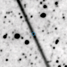
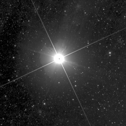
The XMM field would at first seem to fail the 99.9% reliability
requirement in W1 and just barely makes it in W2 (solid curves in the plot).
This is an example of the difficulty in dealing with artifacts from
extremely bright (and possibly variable) sources. The red giant Mira lies
just to the north of the XMM field, as shown in the following images. The
large (partial) circular cutout in the WISE coverage is from the halo, and
the three smaller cutouts are latents.
 |
 |
 |
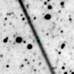
| Figure 28a - Unmatched diffraction spike artifact in the XMM field.
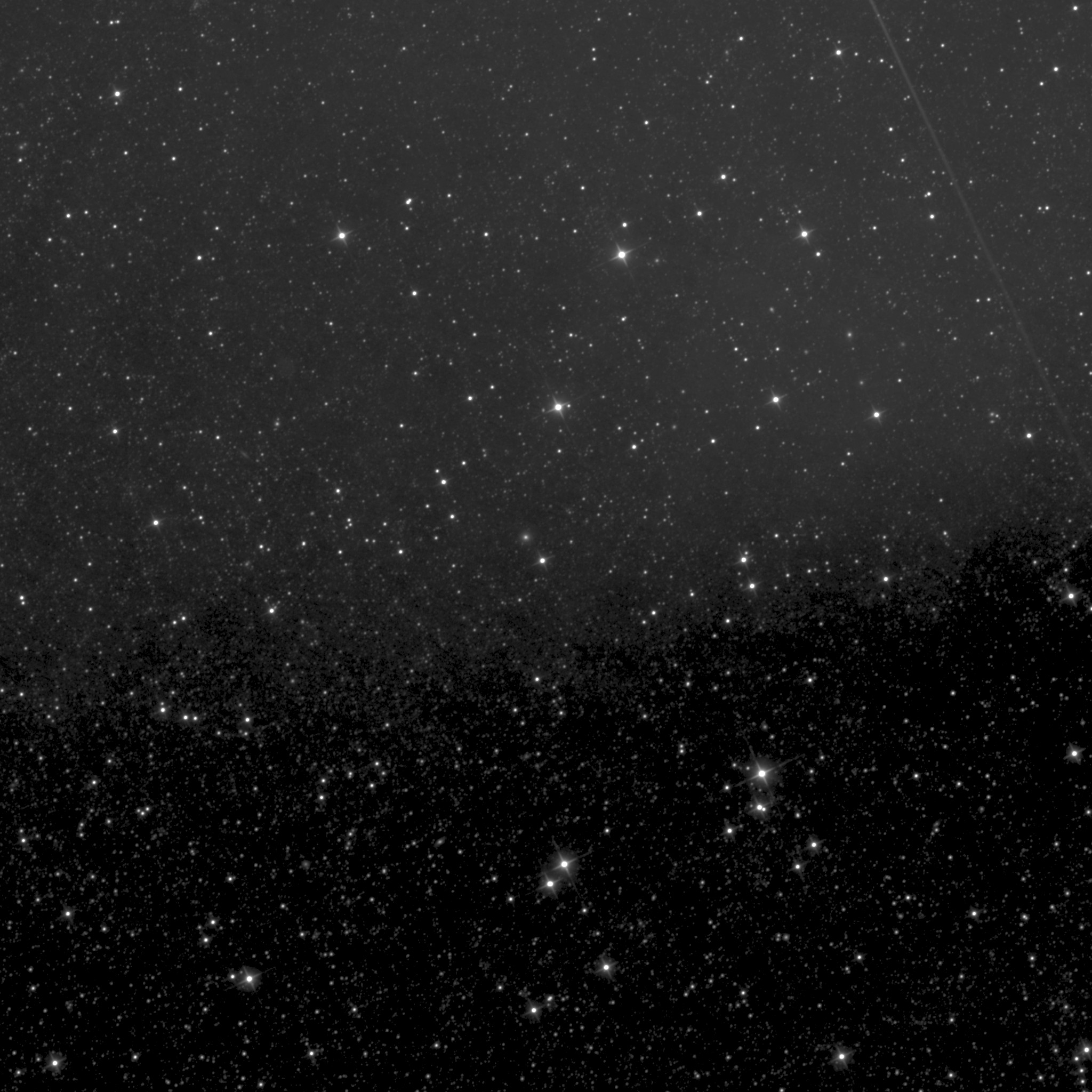
|
Figure 28b - 1.56°x1.56° W1 tile containing Mira.
|
Figure 28c - W1 tile containing the unmatched artifact. The diffraction spike
continues in the upper right corner. |
The images show that the diffraction spikes from Mira extend a
considerable distance away from the star, well over 1.5°, making it
impossible to flag the more remote diffraction artifacts. When these
diffraction artifacts are removed by hand (68 "sources" within the depth
that interactive corrections were done), the dashed curves are produced, and
the reliability of the remaining sources is shown to be well above the
requirement as it was for the other SWIRE fields. Also, the 7 sources with
w3snr ≥ 10 that were not recovered were all sources in the "halo"
surrounding several of the latents. These effects serve as a caveat that
should be noted when working near extremely infrared-bright stars—the
diffraction, halo, and latent models may not reject all possible artifacts,
and visual inspection of the imaging data may be required to ensure an
uncontaminated sample.
Last update: 2012 July 17