Demonstration of the WISE Scan Rate Synchronization Monitor

1. Introduction
2. Method
3. Simulations
1. May 2007 - 21 Image Sequences, 7 Rates
2. June 2007 - Full Orbit with Scan Rate Adjustments
3. July 2007 - Full Orbit with Fine Adjustments, Radiation Hits and Distortion

I. Introduction

This report demonstrates how the standard image quality monitoring segment of WISE Science Data Quality Assurance can be used to track the synchronization of the scan rate and direction of the spacecraft and scan mirror motion, and as a tool to provide information necessary to achieve the initial synchronizization during IOC.

During normal survey operations, WISE will image the sky using a "freeze-frame" scanning technique. While the spacecraft orbits the earth, it executes a continuous pitching maneuver that keeps the telescope boresight pointing near the the zenith. As the telescope field-of-view sweeps the sky, the scan mirror located in the WISE payload moves in the opposite direction to cancel out the apparent motion of the sky. The scan mirror temporarily "freezes" the sky on the WISE focal planes during which time the detectors capture their 8.8 sec exposures on the sky. Following each exposure, the scan mirror flies back to acquire the next field of view and resumes scanning while the detectors acquire images of the new field. This cycle repeats until operations are interrupted for a downlink maneuver or other facility housekeeping operations.

The scan direction and angular rates of the WISE scan mirror and spacecraft must be accurately matched to achieve good image quality. If the rates or directions are mismatched, the sky will not be frozen on the focal planes during the detector exposures, and images of astronomical sources will be smeared as a result. Synchronizing the scan mirror and spacecraft scan rates will be a key activity for WISE during IOC, and monitoring the synchronization during the mission will be an important function of Science Data Quality Assurance (QA).

Standard WISE Science Data QA assessment will include an image quality report that summarizes the mean point source image size and shape measured for individual and groups of WISE science data frames. The WISE image quality QA reporting will be based closely on the 2MASS QA system that monitored image quality as a means to track telescope focus and atmospheric seeing.

The WISE QA image quality assessment is demonstrated here prototype software that has been developed from the 2MASS QA software operating on simulated images that have varying degrees of scan rate mismatching.

II. Method

As in the 2MASS QA system, the WISE Science QA image shape and symmetry report will present in tabular and graphical form mean parameters that indicate if point source images deviate from roundness. Robust image parameters are derived by first combining the images of large numbers of point source detected on one or more image frames to construct high signal-to-noise composite psf images, and then measuring the parameters describing those composite psf's. The general method by which the robust measurements of image parameters are made is as follows:

1. Compile a reference source table for each input image

1. Detect sources in individual image frames.
2. Operationally, the system then selects a subset of detections from each input image that fall in a specified brightest range, and that are extended, not confused with other sources or image artifacts, or that are not otherwised flagged as having corrupted images. For the purpose of this demonstration, though, no filtering was done on the detection list.
2. Generate combined, composite PSF images for each input image

1. Take 9x9 pixel cutouts centered on the position of each reference source. Upsample each pixel in the cutouts 3x3 to generate a 27x27 pixel postage stamp.
2. Combine the postage stamps from each input image to form a composite psf. Combination is done using a two-pass sigma-editing on the stacked pixels values. Operationally, SNR-weighting and other refinements to the combination algorithm may be employed.
3. For this demonstration, two composite psf images were generated for each input image:
   1. A single psf image formed by combining the postage stamps of all reference sources on each input image, and
   2. A 5x5 grid of psf's showing the mean psf images in each of 25 sectors on the array.

   The analysis for this demonstration focuses on the former. The 5x5 psf grids will not be discussed at this time.

3. Measure the asymmetry of the composite psf images for each input image
1. Measure the first and second moments of each image on the composite psf images, and compute the length of the rotated second moment major-axis and its position angle.
2. Fit an ellipse to the 10% power isophote of the composite psf images and determine the ellipse semi-major axis, aspect ratio and position angle.
3. Write image fitting parameters to an output table
4. Generate a web-based and parsable ascii image quality reports as part of the larger QA summary.
1. Link to image fit summary table for a series of images
2. Present graphical representation of measured image size and shape information as a function of frame number
3. Compare measured shape parameters with thresholds and indicate out of spec conditions in concise summary report

III. Simulations

1. May 2007 - 21 Image Sequences, 7 Rates

a. Input Data

Ned Wright supplied two sets of images that simulate the appearance of a sequence of WISE band 1 frames taken with different spacecraft scan rates. Each set was comprised of 21 images, and represented 7 different scan rates (i.e. three frames per scan rate). The first set, denoted "v6" below, incremented the in-orbit (x-direction) scan rate by 0.003'/sec, and the central rate was off by 0.001'/sec in the direction perpendicular to the orbit (y-direction). The step size in the second set, denoted "v7" below, was 0.01'/sec, with no cross-orbit rate error. The images are populated with star images based on a framework of 2MASS All-Sky Point Source Catalog entries. These simulated images are representative of how a sequence of images taken during an IOC task to synchronize the spacecraft scan rate might appear.

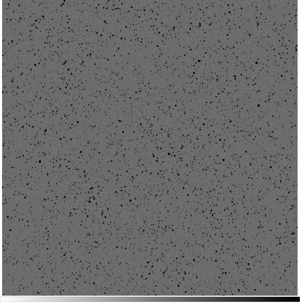
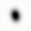
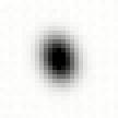
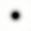
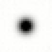
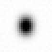
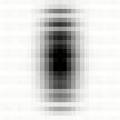
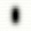
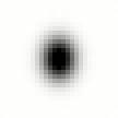
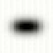
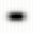
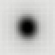
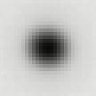
Figure 1 below shows the first image in the "v6" set. The zoomed-in image shown in Figure 2 can be seen to exhibit slightly elongated images implying a mismatch between the spacecraft and scan mirror scan rates and/or directions.

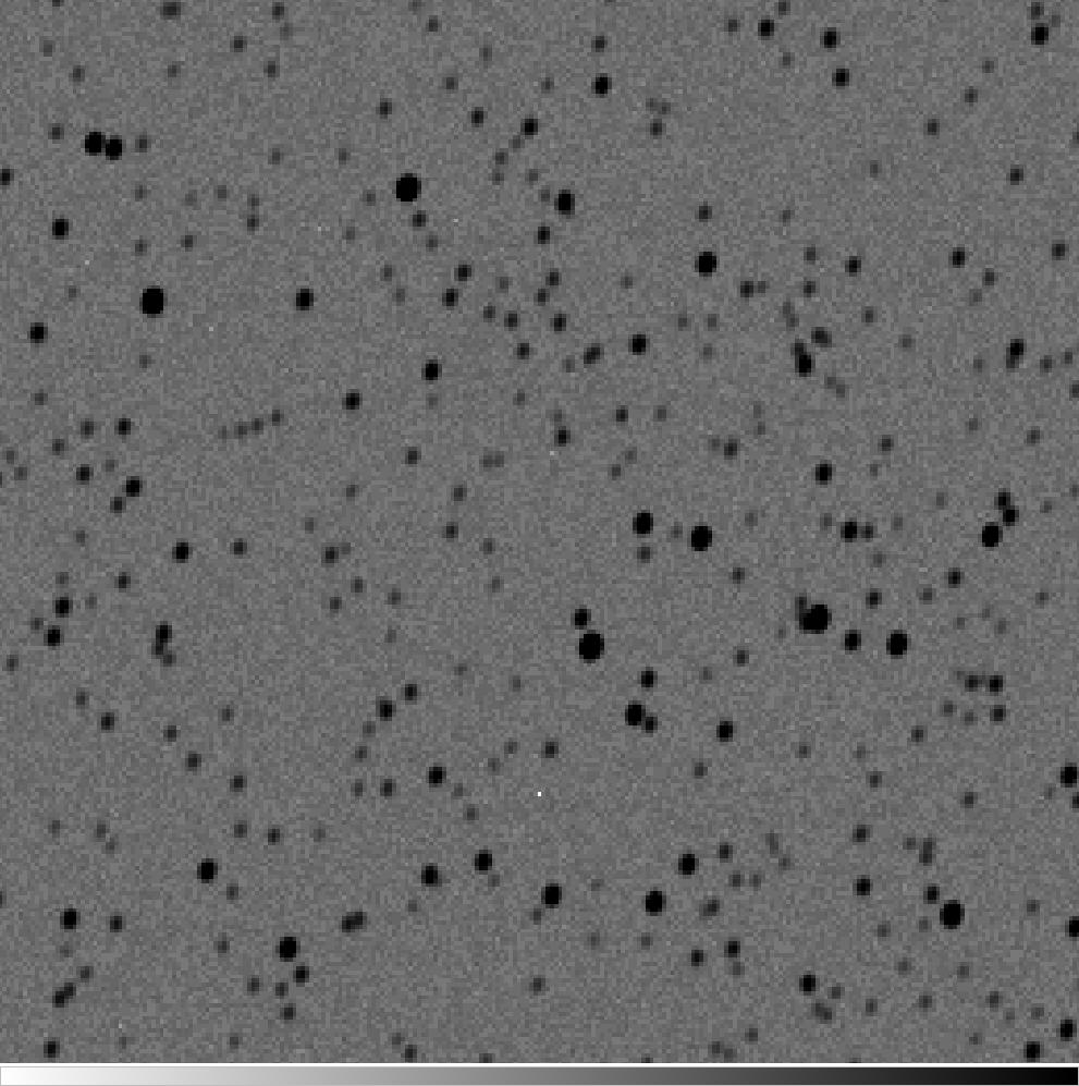Figure 1 - Simulated star-field in the first image of the "v6" sequence.	Figure 2 - Zoom in to Figure 1 showing slight image elongation.

b. Composite PSFs

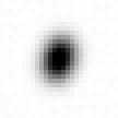
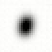
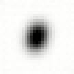
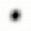
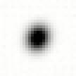
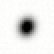
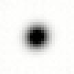
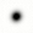
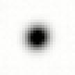
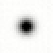
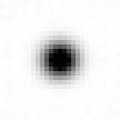
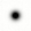
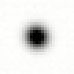
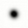
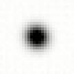
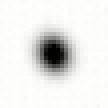
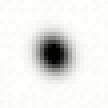
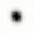
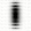
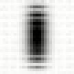
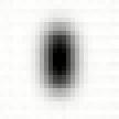
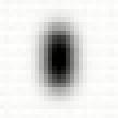
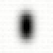
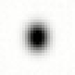
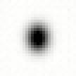
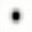
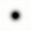
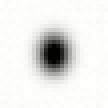
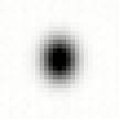
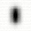
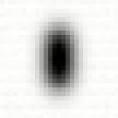
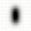
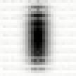
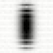
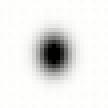
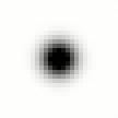
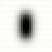
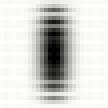
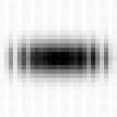
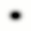
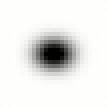
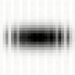
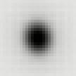
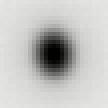
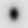
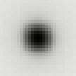
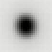
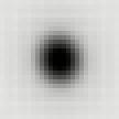
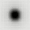
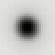
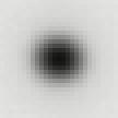
Figures 3-23 show the single composite psf images for the "v6" set. The single composite psf images for the "v7" image set are shown in Figure 24-44. The three composite psf's shown in each row below are taken from the input images with the same scan rate mismatch, and are therefore similar in elongation an position angle. Operationally, composite psf's would be generated by combining source postage stamps from multiple images, thereby improving the effective precision. Composites are developed for the individual images in this simulation to demonstrate repeatability and the minimum capabilities of the algorithm.

The behavior of the composite images in each simulation is similar. The psf's in the first three frames are clearly elongated, then become more symmetric, until the fourth set of three, and then elongate again in the final three sets of three images. The larger scan rate step sizes used between images in the second simulation set ("v7" Figures 24-44) clearly result in more elongated images.

"V6" Simulation Composite PSF Images

Figure 3	Figure 4	Figure 5
Figure 6	Figure 7	Figure 8
Figure 9	Figure 10	Figure 11
Figure 12	Figure 13	Figure 14
Figure 15	Figure 16	Figure 17
Figure 18	Figure 19	Figure 20
Figure 21	Figure 22	Figure 23

"V7" Simulation Composite PSF Images

Figure 24	Figure 25	Figure 26
Figure 27	Figure 28	Figure 29
Figure 30	Figure 31	Figure 32
Figure 33	Figure 34	Figure 35
Figure 36	Figure 37	Figure 38
Figure 39	Figure 40	Figure 41
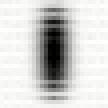Figure 42	Figure 43	Figure 44

c. Composite PSF Image Parameters

Tables 1 and 2 contain the output of the fitting routines used to characterize the single "v6" and "v7" psf images, respectively. The columns in the two tables are as follows:

| par   |   description                                          |
 frame   PSF image name
   x     x-pixel location
   y     y-pixel location
 mom1x   1st moment, x-axis (pixel units)
 mom1y   1st moment, y-axis (pixel units)
 mom2x   2nd moment, x-axis (pixel units)
 mom2y   2nd moment, y-axis (pixel units)
 r_major major axis, rotated-axis 2nd moment (pixel units)
 rb/a    axis ratio from rotated-axis 2nd moment
 rPHI    position angle (EofN) from rotated-axis 2nd moment
 r_0.5p  semi-major axis of the half-power points (arcsec units)
 r_semi  semi-major axis of the 0.1-power points (arcsec units)
 b/a     axis ratio from the 0.1-power points
 PHI     position angle (EofN) from the 0.1-power points

Table 1 - "v6" fitting results	Table 2 - "v7" fitting results

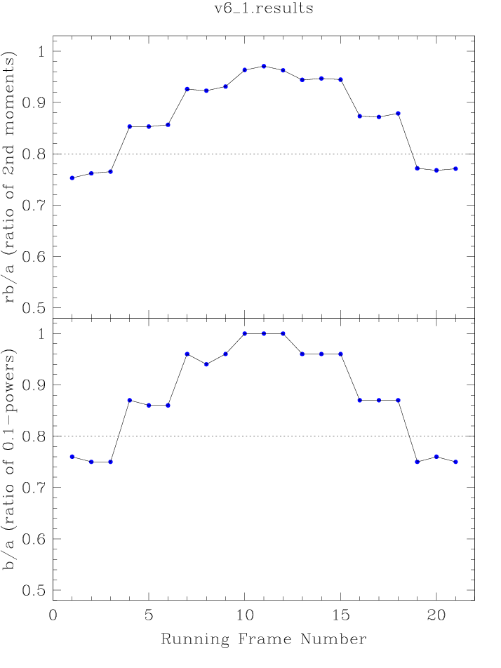
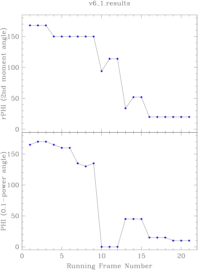
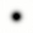
Figures 45 and 46 show the psf image aspect ratio parameters (second moment ratio and 1/10 power ellipse aspect ratio) and their position angles plotted as a function of sequential frame number in the "v6" image set. Each point in the plots corresponds to one of the composite psf images in Figures 3-23. The curves in Figure 45 clearly show that the images are most symmetric 10th-12th images (composite psf's shown in Figures 12-14. Examination of Table 1 shows that the maxima in the image symmetry coincides with the minimum image size (rotated second moment major axis, r_major). The diagrams in Figure 46 quantify the position angle shifts seen clearly in the composite PSF images. Note the position angle rotation through the sequence of images, as might be seen if the spacecraft and scan mirror scan directions are not properly aligned.

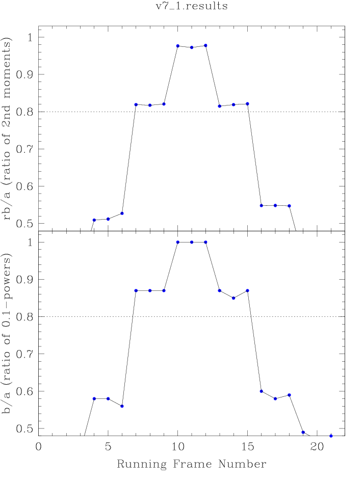
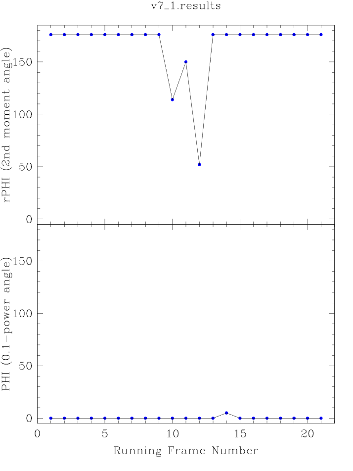
Figures 47 and 48 show the image symmetry parameters and their position angles plotted as a function of sequential frame number in the "v7" image set. Each point in the plots corresponds to one of the composite psf images in Figures 24-44. The curves in Figure 47 show that the images are most symmetric 10th-12th images in the set (composite psf's shown in Figures 33-35. Note that there are little deviations in the measured position angles, suggesting good alignment between the spacecraft and scan mirror directions.

Note that the position angle measurements in both data sets become unreliable when the images become nearly round. Thus, the best way to confirm scan direction alignment is when the scan rates are out of synchronization.

Composite PSF Fit Results

Figure 45 - "v6" PSF Image Aspect Ratio vs. Frame	Figure 46 - "v6" PSF Image Position Angle vs. Frame
Figure 47 - "v7" Image Symmetry vs. Frame	Figure 48 - "v7" Image Position Angle vs. Frame

d. Discussion

The composite psf generation and fitting routines adapted from the 2MASS QA system have been used to demonstrate how WISE image quality will be monitored as part of WISE Science Data QA. This demonstration run on images that simulate data taken with a range of spacecraft scan rates such as might be obtained during IOC shows that the composite image parameter fitting is able to determine the relative image symmetry and size.

Can this diagnostic be used to provide the information to determine when the spacecraft and scan mirror scan rates and directions are matched with sufficient precion? To determine this, the required accuracy should be specified and further simulations developed to test if these diagnostics can measure image parameters with sufficient precision. It is known that the precision of the composite psf's can be increased by combining sources from multiple images, and using refined combination algorithms.

2. June 2007 Simulation - Full Orbit with Scan Rate Adjustments

a. Input Data

486 artifical W1 FITS format images that simulate a scan rate tuning test orbit such as may be executed during IOC were supplied by Ned Wright. The simulated data contain a framework of 2MASS astrometric reference stars with fainter stars added. Each star is modeled with a gaussian point spread function. Instrumental signatures, such as dark current or responsivity variations (i.e. flat-field response) were not added to the images. Frame names have the format "YYDDDHHMMSSS-B.fits", where YY is the year (last two digits), "DDD" is the day of the year, "HHMMSSS" is the UT time and "B" is the band. These images simulate data taken on 11/16/2009 UT, which would be shortly after the WISE cover is ejected for an 11/2/2009 UT launch.

A different tuning run takes place during each half orbit. Each run consists of 7 different scan rates, each executed for 6 minutes of the orbit. Scan rates were specified in an "orbital-events" file, that contains a list of UTC times followed by the commanded scan rate. During actual WISE operations, command information such as scan rate adjustments, will be communicated to the WSDC via the "Significant Orbital Events" (SOE) file as part of the MOS engineering and housekeeping data. The WSDC will parse the SOE file and match events and conditions to time-tagged science data images that are sent from the MOS High Rate Data Processor at White Sands. The "orbital events file" generated for this simulation does not necessarily have the format of the SOE file, but it accurately captures the spirit of how the scan rate information is transferred to the WSDC.

Table 3 contains the UTC times and scan rate settings as indicated in the orbital events file, and the simulated images that correspond to each commanded rate. Scan rates were adjusted in y or orbital direction in the first run, and in the x or orbit-perpendicular direction in the second run. The rates in each direction are indicated as dy and dx, respectively, in units of arcminutes/second.

b. Results

Composite psf's were generated by stacking the images of sources detected in all frames in a test interval that have the same commanded scan rate. As with the previous simulation, no selective filtering of detections was applied. Separate composite psf's were derived for the two different frame intervals with scan rates of dx=3.80'/sec and dy=0.00'/sec (UTC=07:10:51 and 07:57:43 starts).

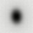
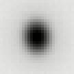
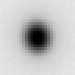
The resulting composite psf's are shown in Figures 49-62. Figures 49-55 represent the x-rate changes and Figures 56-62 are the y-rate changes. Note the 90° position angle shift between the two sets.

Figure 63 is an animated GIF image that shows surface maps of the composite psfs shown in Figures 49-62.

Fig. 49 - dx=3.77,dy=0.00	Fig. 50 - dx=3.78,dy=0.00	Fig. 51 - dx=3.79,dy=0.00	Fig. 52 - dx=3.80,dy=0.00	Fig. 53 - dx=3.81,dy=0.00	Fig. 54 - dx=3.82,dy=0.00	Fig. 55 - dx=3.83,dy=0.00
Fig. 56 - dx=3.80,dy=-0.03	Fig. 57 - dx=3.80,dy=-0.02	Fig. 58 - dx=3.80,dy=-0.01	Fig. 59 - dx=3.80,dy=0.00	Fig. 60 - dx=3.80,dy=0.01	Fig. 61 - dx=3.80,dy=0.02	Fig. 62 - dx=3.80,dy=0.03

Figure 63 - Animated GIF image showing changes in composite psf as scan rate is changed

Table 4 contains the composite psf fitting results. The fitting procedure and output table columns are as described above. The in-orbit and cross-orbit scan rates have been added to each line in the table.

Table 4 - Composite PSF Fit Parameters

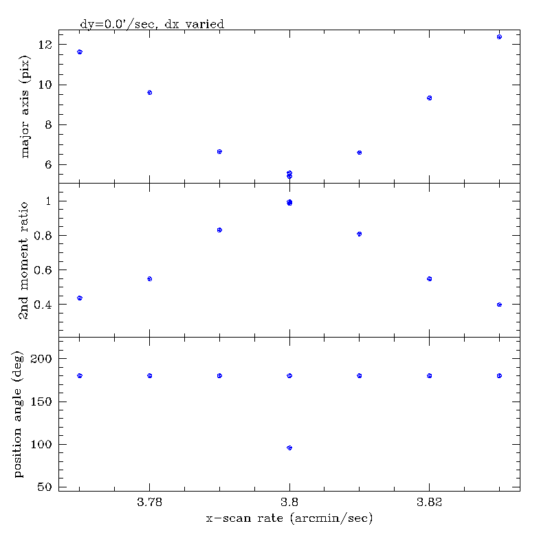
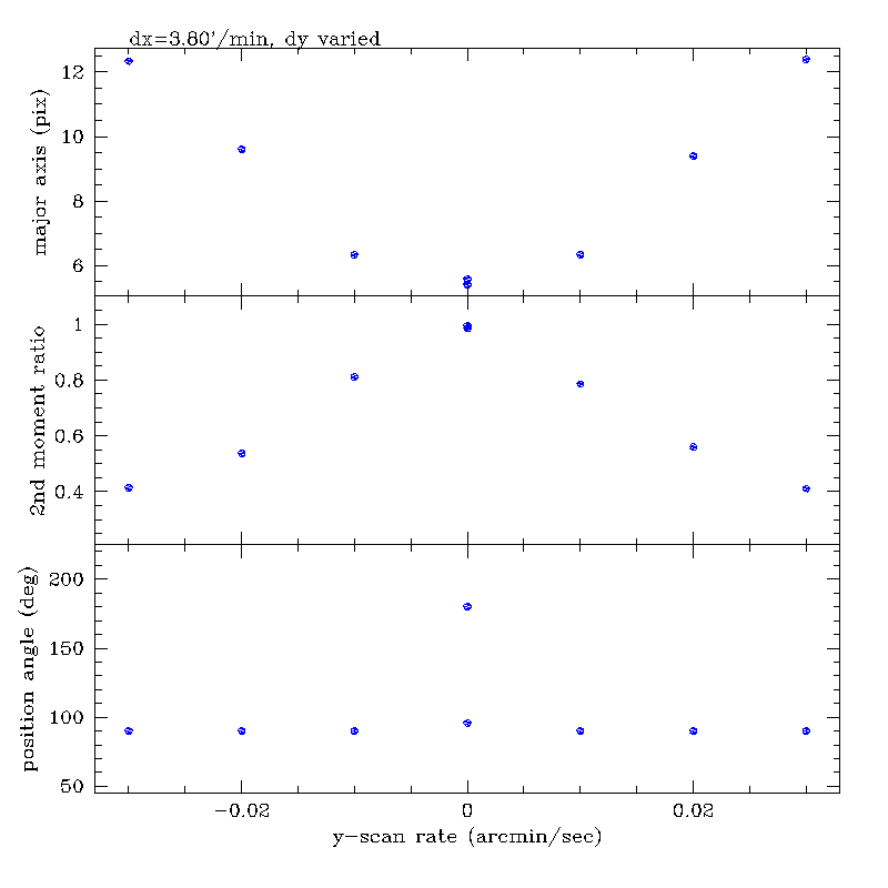
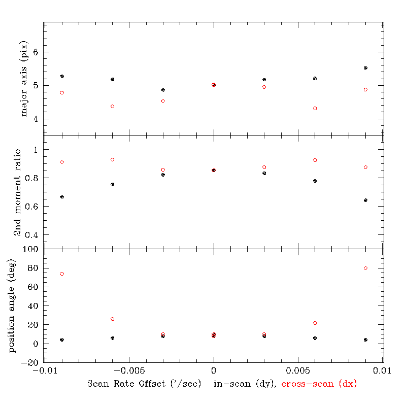
The composite psf semi-major axis size, aspect ratio and position angles plotted as a function of x- and y- scan rates are shown in Figures 64 and 65. The parameters plotted are taken from the second moment fits listed in Table 5. Figure 64 shows the results of varying the x-scan rate while holding the y-scan rate fixed (at 0.0'/sec). Figure 65 shows the results of varying the y-scan rate while holding the x-scan rate fixed (at 3.80'/sec). The two separate intervals with dx=3.80'/sec and dy=0.0'/sec are plotted separately.

There is a clear minimum in the image size and maximum of the image second moment ratio at dx=3.80'/sec and dy=0.0'/sec. As can be seen in Figure 49-61, the position angle of the rotated second moment ratios are very near 180° when the cross-orbit rate is zero. The measured position angles are near 90° when the in-orbit rate is nominal and the cross-orbit scan rate is varied. Position angle measurements when the composite psf's are most nearly circular are poorly defined.

Image Parameters vs. Scan Rate

Figure 64 - Image Parameters vs. x-scan Rate	Figure 65 - Image Parameters vs. y-scan Rate

3. July 2007 - Full Orbit with Fine Adjustments, Radiation Hits and Distortion

a. Input Data

A set of 497 artifical W1 FITS images that simulate a scan rate tuning run during a single orbit were supplied by Ned Wright. These data use the same naming convention as the June 2007 simulations, and they were also constructed using a framework of 2MASS astrometric reference stars with additional faint stars to complete the scenes. Features of these simulated data include the following:

• The scan rate adjustment step sizes are smaller than in the June 2007 simulation - 0.003'/sec in the in-orbit and cross-orbit directions. The full extent of the scan rate mismatches for this simulation are ±0.009'/sec, which is less than one of the rate adjustement steps used in the June 2007 simulation.
• Star images are modeled using the simulated PRF constructed by Peter Eisenhardt that folds in the distortion caused by the scan mirror travel during an exposure, along with a simple focal plane dependent distortion model.
• Detector noise model
• Diffuse cirrus emission
• Simulated radiation hits. Because the radiation hits were simulated as single pixel events that are much narrower than the WISE PRF, their inclusion corrupted the generation of the composite PRF. This forced us to add a provisional "spike" identifier that enabled the radiation hit detections to be identified and rejected during the composite PRF construction.
• Because of computational limitations, simulated star images are not generated for frames taken while the spacecraft has a high slew rate, during the spacecraft yaw maneuvers near the ecliptic pole passages. These frames were identified by visual inspection and eliminated from the analysis that follows.

Table 5 contains the starting UTC times and scan rates as provided in the orbital events files, and the simulated images that correspond to each commanded rated. Note that the in-orbit (dy) and cross-orbit (dx) scan rates are given relative to the nominal scan rate, rather than as absolute rates as was done in Table 3.

b. Results

Composite psf's were generated by stacking the images of sources detected in all frames in the intervals that have the same commanded scan rate. Unlike previous simulations, selective filtering of detections was applied to reject suspected radiation hits.

Figures 63-69 show the resulting single composite psf's for the images taken with varying in-orbit scan rates, and Figures 70-76 show the composite psf's for the cross-orbit scan rate variations. The fits to the semi-major axis length, second moment ratio and position angle for each of the single composite psfs are plotted as a function of in-orbit and cross-orbit scan rate offset in Figure 77.

Fig. 63 dx=0.000, dy=-0.009	Fig. 64 dx=0.000, dy=-0.006	Fig. 65 dx=0.000, dy=-0.003	Fig. 66 dx=0.000, dy=0.000	Fig. 67 dx=0.000, dy=+0.003	Fig. 68 dx=0.000, dy=+0.006	Fig. 69 dx=0.000, dy=+0.009
Fig. 70 dx=-0.009, dy=0.000	Fig. 71 dx=-0.006, dy=0.000	Fig. 72 dx=-0.003, dy=0.000	Fig. 73 dx=0.000, dy=0.000	Fig. 74 dx=+0.003, dy=0.000	Fig. 75 dx=+0.006, dy=0.000	Fig. 76 dx=+0.009, dy=0.000

Fig. 77 - Single composite PSF fit parameters plotted as a function of in-orbit and cross-orbit scan rate offset

While there is a clear maximum in the plot of the second moment ratio as a function of in-orbit scan rate, it is not possible to identify unambiguously the optimal scan rate based on the the second moment ratio versus cross-orbit rate or either of the semi-major axis curves.

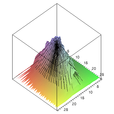
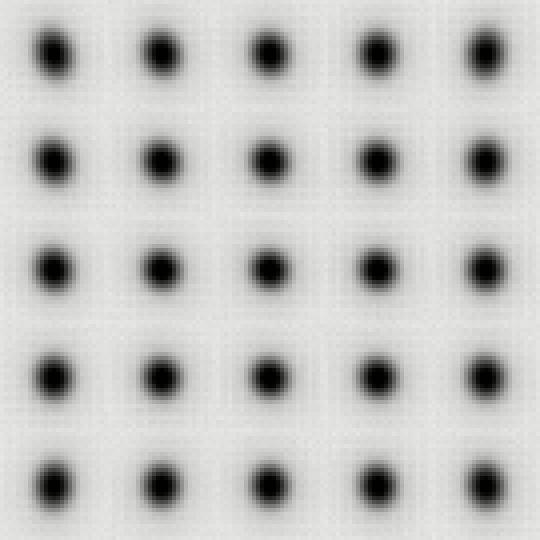
The signature of the scan rate mismatch in the composite psfs is diluted by the effect of image distortion in this simulation. Figure 78 shows a 5x5 grid of composite psfs formed from the images with zero net scan rate offset (e.g. corresponding to Fig. 66). Each of the psfs in this map is generated by combining sources detected in the corresponding subregion of the image. In contrast, the single composite psfs shown in Figures 63-76 are formed by combining images detected all over the focal plane, superimposing the various elongations and position angles, and thus smearing out any subtle effects induced by scan rate mismatch.

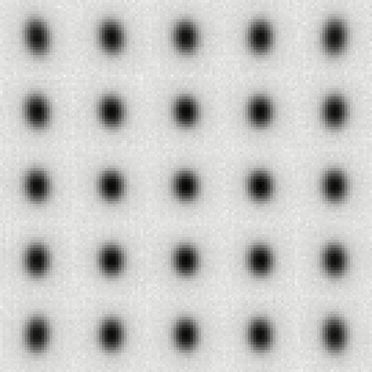
Figure 79 is an animated GIF image that cycles through the 5x5 composite psf maps for each of the scan rate offsets listed in Table 5. The most heavily distorted images in the corners of the maps are circularized when the scan rates are increasingly mismatched, particularly when the mismatch is in the cross-orbit direction. This produces the relatively flat dependence of the second moment ratio on cross-orbit scan rate offset seen in Figure 77.

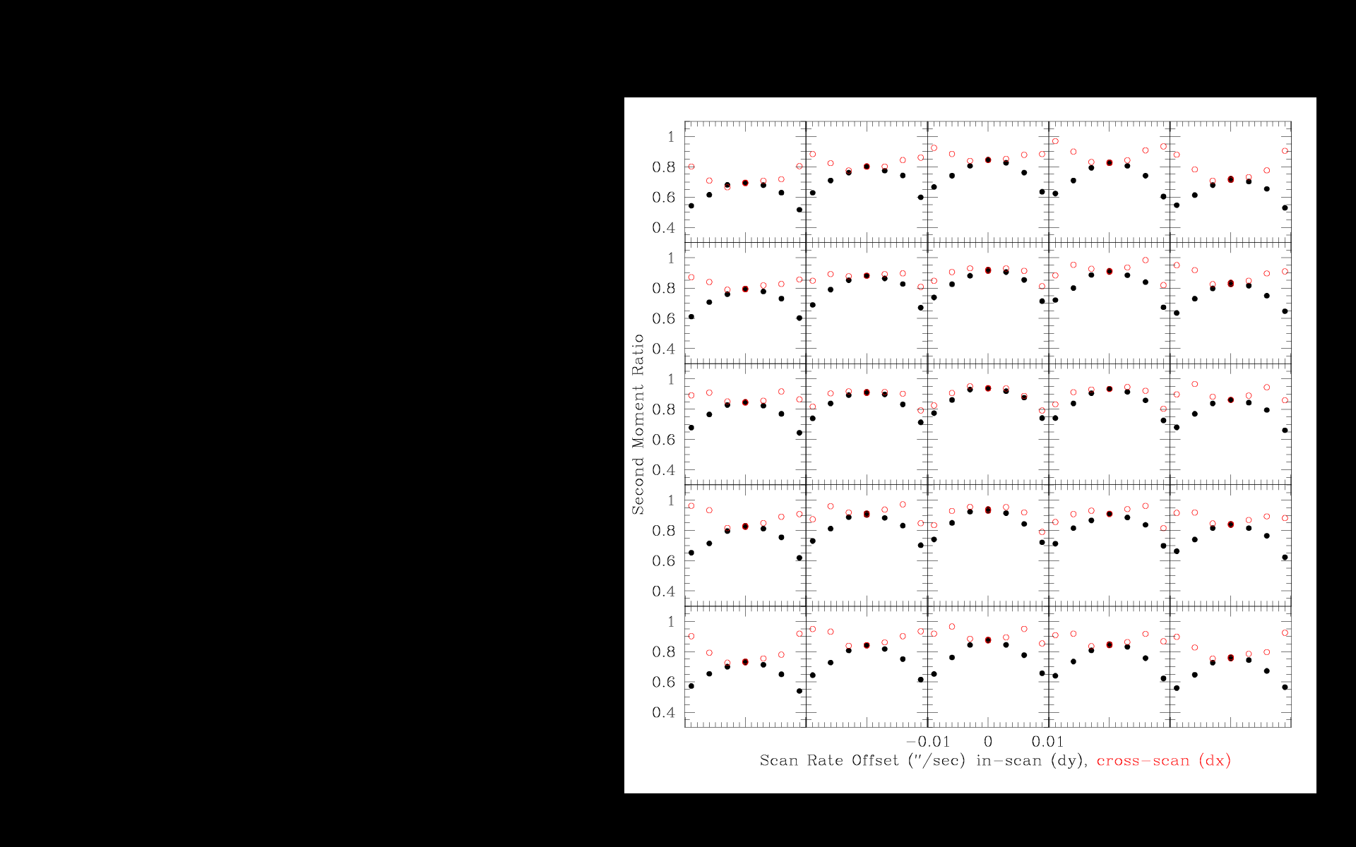
Figures 80 and 81 show the results of fitting the second moment ratio and semi-major axes of each composite psf images in the 5x5 grids, plotted as a function of in-orbit (dy) and cross-orbit (dx) scan rate offsets. The image second moment ratio for is generally useful for diagnosing scan rate mismatches at any point on the focal plan, provided the mismatches are along the orbit direction. If there is a component of scan rate mismatch perpendicular to the orbit direction, then the second moment ratio is useful as a diagnostic only for image data drawn from the central region of the focal plane. In the corners of the focal plane, cross-orbit scan mismatches can actually cause the second moment ratio dependence to invert from what is expected.

Image size (semi-major axis length) is not very sensitive to the relatively small scan rate mismatches used in this simulation. The in-orbit scan rate offset curves suggest that the image size is minimized for a net negative scan rate (-0.003'/sec). The curves of semi-major axis as a function of cross-orbit scan rate offset are not well-behaved, and do not yield an unambiguous identification of optimal scan rate offset.

Fig. 78 - Composite PSF map showing average mean image shape as a function of focal plane position in a 5x5 grid, for dx=0.00, dy=0.00 images.	Fig. 79 - Click on thumbnail to view an animated GIF image that cycles through the 5x5 psf maps for each of the scan rate settings listed in Table 5.	Fig. 80 - Second moment ratio plotted as a function of in-orbit and cross-orbit scan rate offsets for each psf in the 5x5 composite grid.	Fig. 81 - Semi-major axis plotted as a function of in-orbit and cross-orbit scan rate offsets for each psf in the 5x5 composite grid.

c. Conclusions

The results of this simulation are as follows:

• Composite psf image quality can still be used to correctly determine when the spacecraft and scan mirror rates are matched even for relatively small incremental changes in those rates, such as might be used during a "fine tuning" operation
• Some filtering of detections from the science image data will be required to eliminate spurious detections of radiation hits which have significantly sharper profiles than true point source detections
• Optical distortion will dilute the effect of telescope and scan mirror scan rate mismatches on the resulting composite psf behavior. Although it will depend on the actual distortion in the WISE optical system, the best assessment of scan rate matching will be achieved using images of objects detected near the center of the focal planes. In practice, this may require that more images be acquired at a given scan rate so that sufficient number of clean detections of stars are available to form the composite psfs.