


Point Spread Functions (PSFs) for NEOWISE profile-fitting photometry have been estimated from observations of many tens of thousands of stars. Since the PSF shape, Hλ(r), varies significantly over the focal plane due to distortion from the telescope optics, allowance must be made for this effect in the profile-fitting photometry procedure described above. We handle the nonisoplanicity using a library of PSFs corresponding to a 9x9 grid of locations on the focal plane, and then select the appropriate PSF for a given focal-plane location via table lookup.
Each PSF in the library represents an average over a focal-plane segment of width WP, over which we approximate the PSF as locally isoplanatic. The original driver for WP was the WISE Functional Requirement of at least 7% flux accuracy for an unsaturated source with SNR > 100. The 9x9 subdivision of the focal plane exceeds this requirement by typically better than a factor of 4. We now discuss in detail the procedure used for PSF estimation in each focal-plane segment.
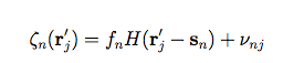
For the particular band, we assume there are N bright star images that fall within the focal-plane segment under consideration. Let ζn(r'j) represent the jth sample of the nth star image after background subtraction and interpolation onto a suitably fine grid r'j (we use a sampling interval of one-eighth of a focal plane pixel); we will use primed coordinates to represent locations on the PSF representation grid in order to distinguish them from focal-plane pixel locations. We assume the original focal plane pixels provide approximately (or better than) Nyquist sampling.
The measurement model for the PSF is then:
 |
(Eq. 1) |
where sn is the location of the nth star in the segment. The origin of the coordinate system for the PSF image is defined to be at the star location.
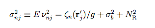
The noise, νnj, is assumed to be an uncorrelated Gaussian random process for which
 |
(Eq. 2) |
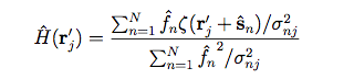
From the set of star images, we can make a maximum likelihood estimate of the PSF using:
 |
(Eq. 3) |
where f^n and s^n represent the estimated flux and position, respectively, of the nth star. For bright stars, an accurate flux estimate can be obtained via aperture photometry.
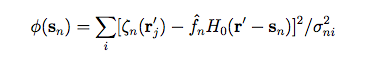
The source position sn is estimated by adjusting the positional offset of the star image for maximum correlation with respect to a nominal starting PSF, H0(r'), for which we used a theoretical form based on optical simulations. The estimation is accomplished by numerical minimization, with respect to sn, of:
 |
(Eq. 4) |
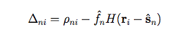
The PSF uncertainty, δH(r), which enters into the photometry noise model, can be estimated by examining the behavior of the data residuals after subtracting a point source model. The ith data residual from the nth star is given by:
 |
(Eq. 5) |
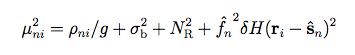
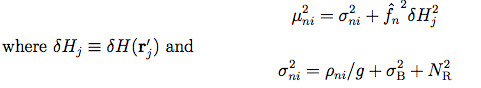
We model Δni as a zero-mean Gaussian random process with variance
 |
(Eq. 6) |
where δH(r) represents the PSF uncertainty at offset r from the PSF origin; g and NR represent the gain and read noise, respectively.
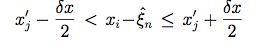
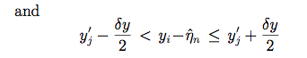
Suppose that the position (ri - sn) falls within the jth pixel on the grid used to represent the PSF, i.e.,
 |
(Eq. 7) |
 |
(Eq. 8) |
where (x'j, y'j) represent the components of r'j, (ξn, ηn) represent the components of sn, and δx, δy represent the sampling intervals of the PSF grid in the x and y directions, respectively.
Then:
 |
(Eq. 9) |
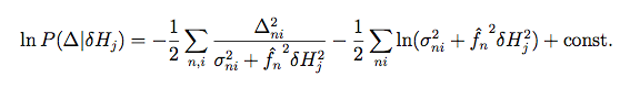
Thus the probability density of the set of local data residuals, Δ, conditioned on δHj, is given by:
 |
(Eq. 11) |
where the summations are overall n, i which satisfy Equations 7 and 8 for a given j.
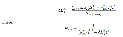
This expression is maximized when:
 |
(Eq. 12)
|
Since δHj is present on both sides of Equation 11, an iterative solution is required. Convergence is rapid, however, and a single iteration suffices.
For each focal plane segment:
The PSFs and their corresponding uncertainty images were generated one band at a time using the procedure described above. Candidate frames were selected from all scans between 45262a and 45300a, taken during the period 17-19 January 2014. Initial frame selection was made by searching source detection tables for unsaturated, uncrowded stars, and requiring SNR of at least 100. Frames were selected to have b > 20 degrees and to be well outside the South Atlantic Anomaly. W1 frames were then individually examined to weed out obvious galaxies, galaxy clusters, satellite trails, very bright stars, diffraction spikes, glints, internal reflections, moon glow, high cosmic ray fluxes, highly structured backgrounds (e.g. nebulae), tracking problems (elongated images), or any image artifacts that might affect the derived PSFs. This selection process left 1030 candidate framesets. The practical limit on the number of frames that WPSFGEN can process at once is ~500, so another 530 framesets were removed in a random fashion. The final list of 500 frames provided 58925 unique sources with SNR > 100.
PSFs were generated in 9x9 grids over the focal plane, with the number of stars ultimately contributing to each PSF ranging between 99 and 283, and with an average of 184 stars per PSF. Following is a set of pseudo color representations of the PSFs using a linear intensity scale, clipped at 60% of peak. The field of view shown for each grid point is 43.5 arcsec across.
 |
 |
||
| Figure 1 - WISE PSFs as a 9x9 spatial grid generated over the focal plane in each band. | |||
Compressed tar files containing the grid of FITS PSF images shown in Figure 1 for each of the bands are available by clicking on the links below:
See the README file for a description of the contents of the files.
Profiles through the central PSF in the 9x9 array in each band are shown in Figure 2. The major axis has been defined as that for which the FWHM is maximized, and the minor axis is taken to be perpendicular to that.
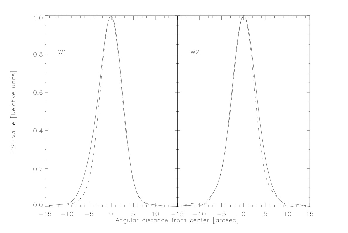
|
| Figure 2 - PSF profiles through major axes (solid lines) and minor axes (dashed lines). |
The major and minor axes and position angles of major axes of the central PSFs are then as follows:
| Band | Major Axis FWHM [arcsec] |
Minor Axis FWHM [arcsec] |
Major Axis PA [deg] |
|---|---|---|---|
| W1 | 6.44 | 5.63 | 56 |
| W2 | 6.70 | 6.09 | 178 |
Noise pixel estimation is described in the section IV.6.c.i of the WISE All-Sky release.
As discussed in section IV.4.c.iii of the WISE All-Sky release, WPRO increases the fitting radius for bright saturated stars, making use of the surrounding annulus of unsaturated pixels. For very bright stars, the saturation region can be larger than the PSF size itself, leaving no usable pixels within the fitting radius. For this reason, we have fitted extended wings to the PSFs. This was accomplished by using the images of bright saturated stars at a large number of positions over the focal plane. There were, however, an insufficient number of such stars to determine the behavior of the PSF wings in all of the 9 x 9 subregions of the focal plane. Yet, just as for the PSF cores, the detailed shapes of the extended wings are seen to vary somewhat with location on the detector. To capture these variations (to the extent possible with a limited number of very bright stars), we grouped stars according to which of the four quadrants on each array they fell in. We then constructed extended PSF wings for each quadrant separately. The outer portions of these extended PSFs were then used to extend the wings of each PSF in the 9 x 9 grid. After some experimentation, all PSFs in the lower-left quadrant (grid locations 01x01 to 04x04) were extended using the wings generated for that quadrant. PSFs in the other quadrants were similarly extended using the appropriate wings. Finally, the inner 3x3 PSFs (04x04 to 06x06) were extended using an average of the extended PSFs from all four quadrants.
The field of view of the resulting augmented PSF images is 3.67 arcmin; this is sufficient to do photometry on even the brightest saturated stars. The resulting PSF images are shown in Figures 3a and 3b below. Corresponding uncertainty maps were derived from the residuals between the average PSF-wing images and the individual bright star images. The outer wings of the resulting PSFs are rather uncertain, and the brightest saturated stars have correspondingly large uncertainties in their quoted magnitudes.
 |
|||
| Figure 3a - Extended wings of W1 PSFs by quadrant. The PSFs are shown on a linear intensity scale, clipped at 0.1% of the PSF peak. | |||
 |
|||
| Figure 3b - As in Figure 3a, but for W2. | |||
Despite the long hibernation and large temperature variations, the PSFs generated for NEOWISE data processing are not very different from those used for AllWISE processing. The W1 PSFs appear to be slightly more elongated (~5%) along the long axis at half-peak intensity, but are virtually unchanged along the short axis. Figure 4 shows curves of growth for the central PSFs for both NEOWISE and AllWISE. The W1 half-light radius has increased from 3.36 to 3.47 arcsec (3%), while the radius containing 80% of the light has increased by 1% to 6.32 arcsec. For W2, the radii containing 50% and 80% of the light have increased by 2.6% and 2.4%, to 3.97 and 7.15 arcsec, respectively.
 |
|||
| Figure 4 - Curves of growth for the central PSFs in both NEOWISE (solid lines) and AllWISE (dashed lines). | |||
Last update: 13 February 2024