


The AllWISE Multiframe pipeline detects sources on the deep coadded Atlas Images, and then measures the sources through PSF-fit photometry using the individual Single-exposures. Optimal source fluxes and positions are measured by fitting pixel data from all available Single-exposure images in all bands simultaneously. The magnitudes in the Source Catalog w?mpro columns are not simply a combination of flux measurements on the individual frames, but rather a simultaneous fit to all pixel data in all bands that makes the best use of all the information.
After the profile-fit extraction for each deep detection source is performed, fluxes are then measured on the individual Single-exposures by solving for the PSF amplitude (i.e. the flux), forced at the sky position of the deep detection fit. These individual frame flux measurements and uncertainties are recorded in the AllWISE Multiepoch Photometry Database (MEP). The Single-exposure fluxes are calibrated and converted to magnitudes using the same procedures, zeropoints, and conventions as are used for the entries in the Source Catalog.
For faint deep detection sources, the individual Single-exposure flux measurements will have SNR<2, and magnitudes in the MEP Database therefore will be upper limits. In addition, the measurements in the MEP Database are limited to only those from Single-exposures that satisfied the quality requirements to be used for the AllWISE Multiframe processing. There may be Single-exposure measurements for images excluded from the AllWISE processing in the All-Sky, 3-Band Cryo, or Post-Cryo Single-exposure Source Working Databases. However, because of the shallower depth of the Single-exposures, the faintest sources may not have been detected, and the corresponding photometry will not be available.
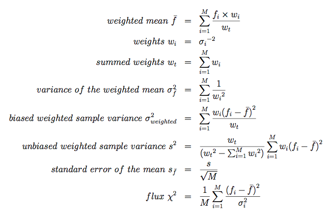
A number of statistics are computed using the distribution of Single-exposure fluxes measured for each deep detection source. Equations 1-8 describe the basic flux distribution moments that are calculated, including the inverse variance-weighted mean, unbiased weighted sample variance and the standard deviation of the mean. For example, the w?magp values in the Source Catalog are magnitudes computed from the inverse variance weighted mean fluxes, and are on average very similar to the deep detection profile-fit magnitudes, as illustrated in Figures 5a-d in II.1.d.i. All of the Single-exposure flux distribution statistics and related parameters included in the Source Catalog and Reject Table are described in Table 1. These statistics are particularly useful for identifying and classifying flux variability, as described in V.3.b.vi.
Note that fluxes measured for saturated sources during the Post-Cryo phase of the mission are not used in the calculation of flux distribution statistics because of the positive flux bias (II.1.d.i.). These measures are included in the MEP Database, however.
 |
(Eq. 1)
|
Here M is the total number of measurements, fi is the flux of the ith measurement, wi is the weight of the ith element, wt is the sum of the weights.
| Column Name | Description | |
|---|---|---|
| w?m | The number of individual frames that are available to make a deep detection profile-fit measurement in band "?", where "?" = 1, 2, 3, or 4. | |
| w?nm | The number of individual frames on which WPRO extracted a flux measurement with SNR > 3. | |
| w?magp | Sigma-clipped and inverse variance-weighted integrated flux in magnitude units, in each band. | |
| w?sigp1 | Unbiased, weighted sample standard deviation in magnitude units (1.0857*sqrt(Equation 6)/Equation 1). | |
| w?sigp2 | Standard deviation of the mean flux in magnitude units (1.0857*Equation 7/Equation 1). | w?k | Stetson K-index (Stetson, P. 1996, PASP, 108, 851), which provides a robust measure of the kurtosis of the magnitude histogram in the band. The value of w?k tends to 1.0 when the variability is much larger than the uncertainties in individual observations, and to 0.798 when the photometric errors dominate over real variations. |
| w?ndf | Number of degrees of freedom in the flux variability chi-square in band "?". This quantity is used for pre-filtering in the variability flag computation. | |
| w?mlq | Probability measure that the source flux is variable in band ?. The value is -log10(Q), where Q = 1-P(chi2). P is the cumulative distribution probability for flux[1]. The value is clipped at 9. This quantity is used as a component in the variability flag computation. | |
| w?mjdmin | The minimum modified Julian Date (mJD) of the frames used in the flux distribution computation in each band. | |
| w?mjdmax | The maximum modified Julian Date (mJD) of the frames used in the flux distribution computation in each band. | |
| w?mjdmean | The mean modified Julian Date (mJD) of the frames used in the flux distribution computation in each band. | |
| rho12 | The correlation coefficient between the W1 and W2 single-frame flux measurements. The value is a signed 2-digit integer, expressed as a percentage. Negative values indicate anticorrelation. This quantity is used as a component in the variability flag computation. Rho12 is equal to 100 times the J variability index of Stetson (1996 PASP, 108, 851) computed for W1 and W2. | rho23 | The correlation coefficient between the W2 and W3 single-frame flux measurements. The value is a signed 2-digit integer, expressed as a percentage. Negative values indicate anticorrelation. This quantity is used as a component in the variability flag computation. Rho23 is approximately equal to 100 times the J variability index of Stetson (1996 PASP, 108, 851) computed for W2 and W3. | rho34 | The correlation coefficient between the W3 and W4 single-frame flux measurements. The value is a signed 2-digit integer, expressed as a percentage. Negative values indicate anticorrelation. This quantity is used as a component in the variability flag computation. Rho34 is approximately equal to 100 times the J variability index of Stetson (1996 PASP, 108, 851) computed for W3 and W4. | q12 | Correlation significance between W1 and W2[2]. The value is -log10(Q2(rho12)), where Q2 is the two-tailed fraction of all cases expected to show at least this much apparent positive or negative correlation when in fact there is no correlation. The value is clipped at 9. This quantity is used as a component in the variability flag computation. | q23 | Correlation significance between W2 and W3[2]. The value is -log10(Q2(rho23)), where Q2 is the two-tailed fraction of all cases expected to show at least this much apparent positive or negative correlation when in fact there is no correlation. The value is clipped at 9. This quantity is used as a component in the variability flag computation. | q34 | Correlation significance between W3 and W4[2]. The value is -log10(Q2(rho34)), where Q2 is the two-tailed fraction of all cases expected to show at least this much apparent positive or negative correlation when in fact there is no correlation. The value is clipped at 9. This quantity is used as a component in the variability flag computation). |
| Notes to Table 1: [1] The Q value is the fraction of all cases to be expected if the null hypothesis is true. The null hypothesis is that the flux is emitted by a non-variable astrophysical object. It may be false because the object is variable. It may also be false because the flux measurement is corrupted by artifacts such as cosmic rays, scattered light, etc. The smaller the Q value, the more implausible the null hypothesis, i.e., the more likely it is that the flux is either variable or corrupted or both. [2] When the number of measurements is large, the significance of correlation also tends to be large even though the correlations themselves may have a relatively small magnitude. This is a typical manifestation of statistical significance increasing as the sample size increases; eventually the high significance can be due to small correlated errors in background estimation or even roundoff errors. These effects tend to be small but become significant when there are enough observations of them. High flux correlation significance should be taken seriously only when the magnitude of the correlation is also fairly high. | ||
Last update: 4 December 2018