IV. WISE Data Processing

6. Quality Assurance (QA)

a. Steps in QA

ii. ScanFrame QA

ii.1. Scan-level QA checks

ii.1.1. Scan-level metrics

Factors qs1, qs5, and qp were determined per scan and were the basis of the Scan Quality (SQ) score. SQ was the minimum of the qs1, qs5, and qp factors multiplied by ten. SQ was an integer of value 0 (poor quality), 5, or 10 (high quality).

qs1: This was the quality of scan synchronization as judged from the overall 1x1 PSF grid computed by the PSF Moments routine and evaluated based on the effective number of noise pixels (NoisePix). The overall value of qs1 was taken to be the lowest qs1 value of the four bands, computed as follows:

W1:
qs1=1.0 if NoisePix ≤ 13.5 pixels
qs1=0.5 if 13.5 < NoisePix ≤ 14.5
qs1=0.0 if NoisePix > 14.5

W2:
qs1=1.0 if NoisePix ≤ 15.5 pixels
qs1=0.5 if 15.5 < NoisePix ≤ 18.2
qs1=0.0 if NoisePix > 18.2

W3:
qs1=1.0 if NoisePix ≤ 36.6 pixels
qs1=0.5 if 36.6 < NoisePix ≤ 48.4
qs1=0.0 if NoisePix > 48.4

W4:
qs1=1.0 if NoisePix ≤ 27.3 pixels
qs1=0.5 if 27.3 < NoisePix ≤ 34.0
qs1=0.0 if NoisePix > 34.0

qs5: This was the quality of scan synchronization from the 5x5 PSF grid, also computed by the PSF Moments routine and evaluated based on the effective number of noise pixels (NoisePix). The overall value of qs5 was taken to be the lowest qs5 value of the four bands, computed as follows:

W1:
qs5=1.0 if NoisePix ≤ 13.5 pixels
qs5=0.5 if 13.5 < NoisePix ≤ 17.4
qs5=0.0 if NoisePix > 17.4

W2:
qs5=1.0 if NoisePix ≤ 15.5 pixels
qs5=0.5 if 15.5 < NoisePix ≤ 21.8
qs5=0.0 if NoisePix > 21.8

W3:
qs5=1.0 if NoisePix ≤ 36.6 pixels
qs5=0.5 if 36.6 < NoisePix ≤ 58.1
qs5=0.0 if NoisePix > 58.1

W4:
qs5=1.0 if NoisePix ≤ 27.3 pixels
qs5=0.5 if 27.3 < NoisePix ≤ 40.8
qs5=0.0 if NoisePix > 40.8

qp: This was the quality of the photometric zero-point offset computed using profile-fit photometry (pzp). The value of qp was 1.0 for a frameset passing the following criteria; otherwise the value was 0.0:

W1: -0.083 mag < pzp < +0.050 mag
W2: -0.063 mag < pzp < +0.015 mag
W3: -0.012 mag < pzp < +0.186 mag
W4: -0.469 mag < pzp < +0.370 mag

ii.1.2. Scan-level checks

In the following discussion, scan 01432a is used to illustrate the kinds of tabular and graphical material used by QA scientists to assess further the quality of the ScanFrame data.

General: The first section of the web interface contained information about whether the scan successfully completed processing, the number of failed framesets if processing problems were encountered, information about the scan position on the sky (Figure 1), and the number of objects detected (Figure 2).

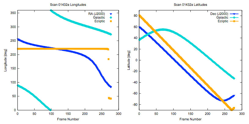Figure 1 - Left: Plot of Right Ascension (dark blue), Galactic longitude (cyan), and ecliptic longitude (orange) as a function of frame number along the scan. Right: Plot of Declination (dark blue), Galactic latitude (cyan), and ecliptic latitude (orange) along the scan. Note that this scan crosses the south ecliptic pole.

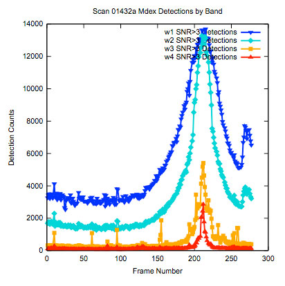Figure 2 - The number of detections per band as as function of frame number along the scan. W1 is shown in dark blue, W2 in cyan, W3 in orange, and W4 in red. Note the spike in the number of detections around frame number 215 when the scan crosses the Galactic plane (see Figure 1).

Instrumental calibration: The Instrumental Calibration section of the QA web interface displayed, as a function of frame number and separately for each band, various metrics related to the background signal, noise, bad pixel counts, focal array temperature, and time since the most recent anneal.

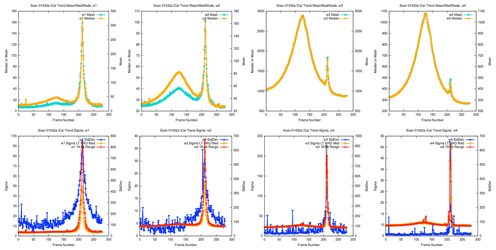Figure 3 - The first row of plots displays the mean (cyan) and median (orange) signal level for each frame. The sharp spike in signals around frame 215 results from crossing the galactic plane. The broader spike around frame 120 results from crossing the ecliptic plane. The second row of plots shows three different noise measurements for each frame: standard deviation (dark blue); low-tail median absolute deviation from median, after iterative trimming of the upper tail of the distribution (orange); and standard deviation in the 16--84 percentile of the distribution (red).

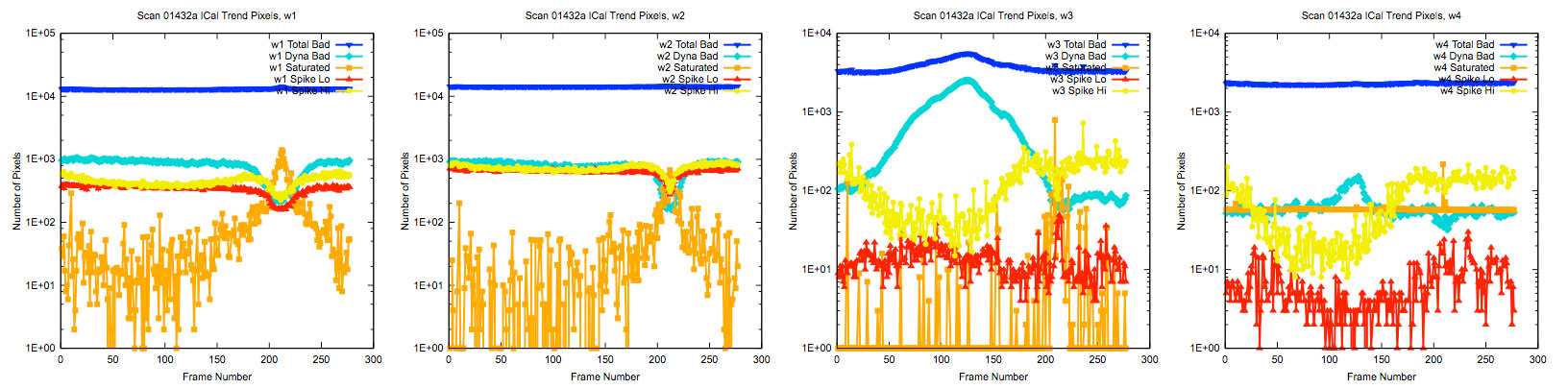Figure 4 - The number of bad pixels for each frame. The values plotted are the total number of bad pixels (dark blue), which is the sum of the other four quantities shown; the number of dynamically-tagged bad pixels (cyan); the number of saturated pixels (orange); the number of low or downward spike pixels (red); and the number of high or upward spike pixels (yellow).

Image quality: The WISE spacecraft was in constant motion and an internal scan mirror countered this motion to allow for a fixed location of the scan to be observed. Image quality depended on how well this scan mirror was synchronized with the spacecraft motion; a scan mirror that is out of synchronization would result in streaked stars. Throughout the mission, several other reasons for poor image quality were also identified: excessive moon light in the star trackers, excessive cosmic rays in the star trackers while in the SAA, and slight changes in spacecraft motion caused, for example, by momentum dumping and spacecraft settling after TDRSS passes. The image streakiness varied from mildly elliptical stars to, in severe and rare cases, stars smeared over several arcminutes.

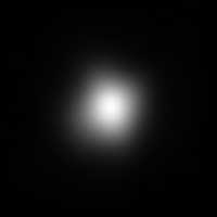
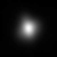
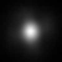
The primary method of tracking image quality was to examine the PSFs of stars in both the individual frames and the scans as a whole. The main products were images of the composite PSFs (Figures 5a-d) and tables describing these PSFs numerically (Table 1).

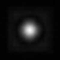Figure 5a - W1 PSF for scan 01432a	Figure 5b - W2 PSF for scan 01432a	Figure 5c - W3 PSF for scan 01432a	Figure 5d - W4 PSF for scan 01432a

The columns in the table are given below. Additional discussion on these quantities can be found in the PSF Moments section.

• scan_id: scan identifier
• band: W1, W2, W3, or W4
• r_major: semi-major axis
• rbovera: axis ratio
• rphi: position angle, measured counterclockwise from the y-axis
• r_05p: semi-major axis of the half-power points
• r_01p: semi-major axis of the 1/10th power points
• bovera: axis ratio from the 1/10th power points
• phi: position angle from the 1/10th power points, measured counterclockwise from the y-axis
• noisepix: effective number of noise pixels
• signspix: 1-σ uncertainty of noisepix
• sigrmajor: 1-σ uncertainty of semi-major axis (r_major)
• sigphi: 1-σ uncertainty of the position angle (rphi)
• sigbovera: 1-σ uncertainty of the axis ratio (rbovera)

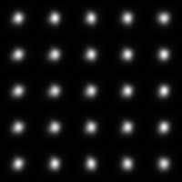
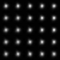
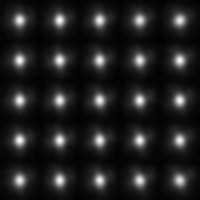
The PSF was also tracked as a function of position on the array to look for image degradation in the corners of the arrays. For this, the array was divided into twenty-five sections (a 5x5 grid), and the PSF computed using stars within each section. Figures 6a-d show the 5x5 PSFs for scan 01432a. A table with the PSF moments for each of the 25 image sections and each band was also computed but is not shown here.

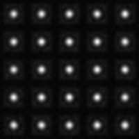Figure 6a - W1 5x5 PSF grid for scan 01432a	Figure 6b - W2 5x5 PSF grid for scan 01432a	Figure 6c - W3 5x5 PSF grid for scan 01432a	Figure 6d - W4 5x5 PSF grid for scan 01432a

Astrometric calibration: Monitoring of WISE astrometry used both internal and external checks to look for potential problems.

2MASS stars were used as the basis for position reconstruction. By monitoring the number of 2MASS stars used in each frame (Figure 7), frames with extremely poor positional reconstruction, as seen via an anomalously low number of positional calibrators, could be flagged. In this example, the number of positional calibrators varied smoothly, showing the expected rise and plateau around the Galactic plane, and no problems were seen.

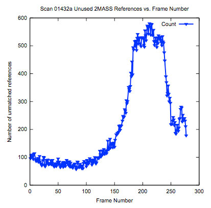Figure 7 - The number of 2MASS reference stars used in the astrometric solution as a function of frame number.

The initial astrometric solutions were based on the expected frame center positions as commanded to the telescope. These could be off by several arcminutes from the frame centers of the final solution, but in all cases this should have been a small fraction of the field-of-view. Figure 8 shows the typical differences for Right Ascension, Declination, and position angle between the final astrometric solution using the 2MASS reference stars and the initial solution using the commanded position information. Large excursions relative to nearby framesets could indicate problems with the astrometric solution or the pointing of the telescope.

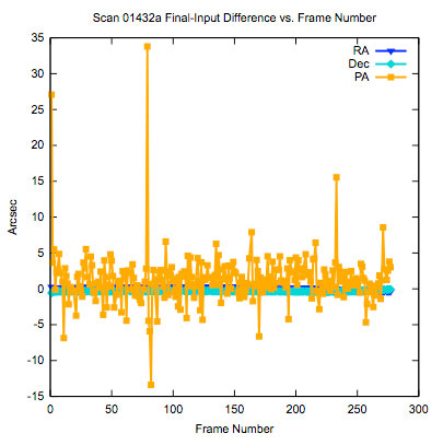Figure 8 - Offsets between final and initial astrometric solutions

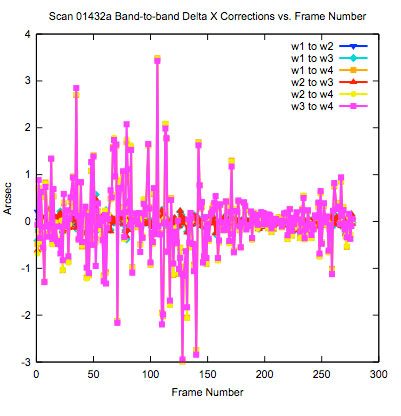
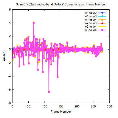
Although the final astrometric calibration was applied to all bands in a frameset, there were variations in the amount of the correction that needed to be applied to a single-frame solution to rectify it with the four-band solution. Figures 9a-c show the band-to-band offsets in X (approximately ecliptic longitude), Y (approximately ecliptic latitude), and rotation angle for scan 01432a. As expected, the average differences are centered around zero for each of these quantities. W4 shows the largest differences with the other bands primarily because of the larger native pixel scale and the relative dearth of 2MASS stars that can be used in the position reconstruction.

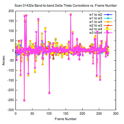Figure 9a - Band-to-band differences in X	Figure 9b - Band-to-band differences in Y	Figure 9c - Band-to-band differences in θ

Photometric calibration: Most scans cross either the north or south ecliptic pole where the WISE photometric calibrator stars are located. For these sources, the WISE-measured PSF magnitudes were taken from the scan's source lists and compared to cataloged magnitudes. The difference between the cataloged and scan-measured (aka "instrumental") magnitudes was the per-scan determination of the photometric zero-point. The scan's measured zero-point was then compared to the average zero-point based on the first month of WISE data to look for any gross changes in detector responsivity. (See the thresholds set for the qp factor.) Plots in support of this check are shown in Figure 10.

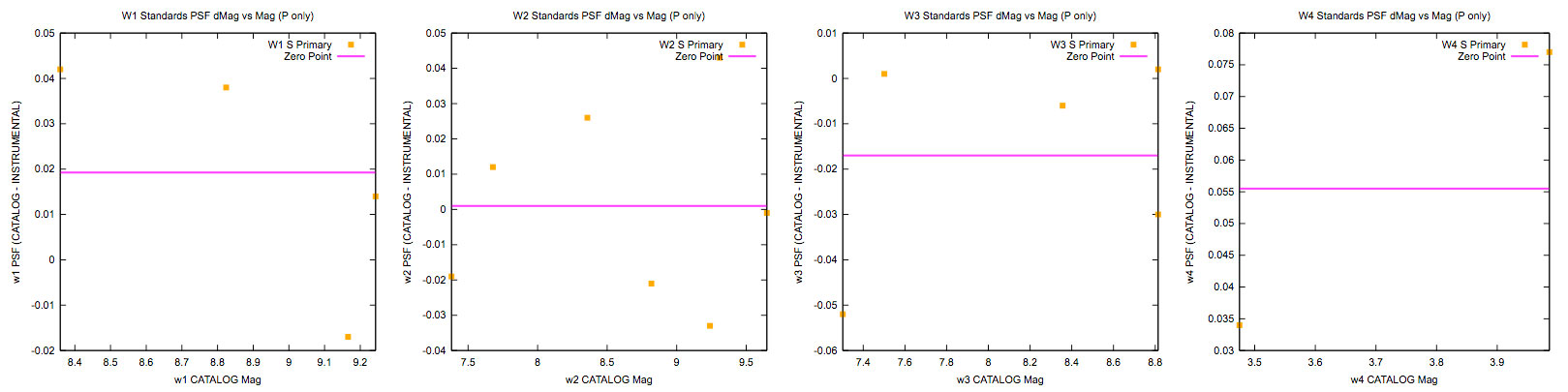Figure 10 - The difference (orange points) between the cataloged magnitude and the PSF magnitude measured in this scan for photometric calibrators at (from left to right), W1, W2, W3, and W4. The measured zero-point offset in each band is shown by the magenta line. This scan crosses only the south ecliptic pole so only southern calibrators are present.

The QA interface also monitored changes in the zero-point along the course of the scan by comparing the extracted profile-fit magnitudes of the same objects seen in the overlap region between consecutive frames. Figure 11 confirms that there is no change in the photometric zero-points along the course of this scan.

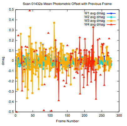Figure 11 - The mean photometric offset for stars in the overlap region between consecutive frames as measured in W1 (dark blue), W2 (cyan), W3 (orange), and W4 (red). Fewer sources in W3 and W4 translate into larger measurement uncertainties for these bands, compared to W1 and W2. Note that the mean offset is 0.0 mag throughout, indicating stable detector responsivity.

Frame statistics: Successive frames in a scan were required to overlap by at least 5%. Because (a) the rotation between successive framesets was minimal, (b) successive framesets had approximately the same ecliptic longitude at their centers, and (c) the pixel scale was constant, the percentage of overlap between two successive frames could be assumed to be inversely proportional to the distance separating the frame centers. (For a case of significant rotation with respect to ecliptic longitude, this estimate could in principle be overestimated by as much as 16%. Therefore, we lowered the 5% overlap requirement by 16%, to 4.2%.) The computation for frame-to-frame overlap was:

• compute the radial distance between a frame and the one immediately prior using the frame centers (this is the quantity d)
• The maximum overlap between the two frames is then given by a_max = 1 - d/l, where l is the length of the array in the same units as d.
• a_max needs to be normalized because of possible rotation issues. So, a_norm = a_max - (a_max * 0.16) = a_max * 0.84 .

The corresponding plot showing frame-to-frame overlaps along the course of scan 01432a is shown in Figure 12. The amount of overlap (approximately 8.6%) is typical for most scans. This plot also shows a "blip" around frame 75. These blips occurred occasionally and were attributed to small attitude adjustments in the spacecraft pointing. In nearly all cases of spacecraft attitude adjustments, the image quality was degraded and the stars were noticably streaked on or near that frame.

Figure 12 - Percentage of array overlap between a given frame and the previous frame.

Solar system objects: Astrophysical results were also used as further checks of the integrity of the data. In this example (Figure 13), the association of WISE sources to the predicted positions of known solar system objects was used as a further check that the astrometric reductions were sound. Figure 13 verifies that, as expected, hundreds of asteroids are successfully matched along the ecliptic plane.

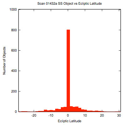Figure 13 - A histogram of the ecliptic latitude distribution of solar system objects successfully matched to WISE detections throughout the course of this scan.

Visual checks: As a final check of data integrity for the scan as a whole, QA scientists visually inspected the images in all bands. The QA interface presented jpeg thumbnails of each frame (Figures 14 and 15), the visual inspection of which would occasionally reveal problems not captured by the QA metrics.

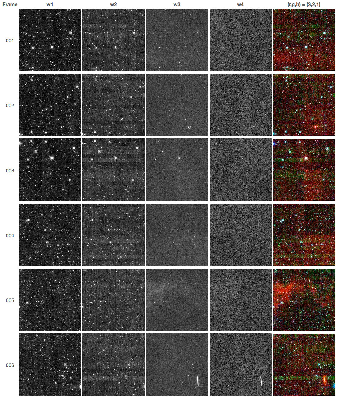Figure 14 - JPEG thumbnails of the first six framesets in the scan. From left to right are shown the W1, W2, W3, W4 and three-color images. The three-color image is a combination of W1 (blue), W2 (green), and W3 (red) frames. These frames fall in a region of moderate stellar density.

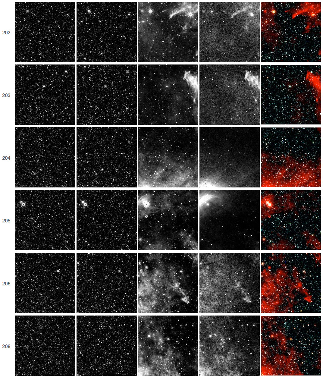Figure 15 - JPEG thumbnails of a high source density region along the Galactic plane. From left to right are shown the W1, W2, W3, W4 and three-color images. The three-color image is a combination of W1 (blue), W2 (green), and W3 (red) frames.

Last update: 2012 January 23